
Self-Driving Car Engineer Nanodegree
Deep Learning
Project: Build a Traffic Sign Recognition Classifier
An important part of self driving cars is the detection of traffic signs. Cars need to automatically detect traffic signs and appropriately take actions. However, traffic sign detection is a difficult problem because of the absence of any standard whatsoever. Different countries have different traffic signs and they mean different things. Weather plays an important role in the presence traffic signs. A very good example of this would be a place which gets heavy snow vs a place which is hot and has deserts around it. Traffic rules and signs around such places are different and hence need to be identified differently.
This was the 2nd project for the Udacity’s Self Driving Car Nanodegree. The problem set provided training and testing data for traffic signs.
For the purpose of this project, Udacity made it a little easier and provided a zip file with test, validation & training data. The zip file contained 3 different pickle files for each.
- train.p - Training Data with 34799 images of each 32x32x3
- valid.p - Validation Data with 4410 images of each 32x32x3
- test.p - Testing Data with 12630 images of each 32x32x3
Step 0: Load The Data
# Load pickled data
import pickle
import pandas as pd

# Augmented Data is stored here
# https://s3-us-west-1.amazonaws.com/traffic-sign-augmented-data/augmented.p

# TODO: Fill this in based on where you saved the training and testing data
use_augmented = False

if use_augmented:
    training_file = 'augmented/augmented.p'
else:
    training_file = 'data/train.p'

validation_file= 'data/valid.p'
testing_file = 'data/test.p'

with open(training_file, mode='rb') as f:
    train = pickle.load(f)
with open(validation_file, mode='rb') as f:
    valid = pickle.load(f)
with open(testing_file, mode='rb') as f:
    test = pickle.load(f)

X_train, Y_train = train['features'], train['labels']
# X_valid, Y_valid = valid['features'], valid['labels']
X_test, Y_test = test['features'], test['labels']

from sklearn.model_selection import train_test_split

X_train, X_valid, Y_train, Y_valid = train_test_split(X_train, Y_train, test_size=0.2, random_state=0)

print("Updated Image Shape: {}".format(X_train[0].shape))

frame = pd.read_csv('signnames.csv')

def get_signname(label_id):
    return frame["SignName"][label_id]
Updated Image Shape: (32, 32, 3)
Step 1: Dataset Summary & Exploration
### Replace each question mark with the appropriate value.
### Use python, pandas or numpy methods rather than hard coding the results
import numpy as np

# TODO: Number of training examples
n_train = train['features'].shape[0]

# TODO: Number of testing examples.
n_test = test['features'].shape[0]

# TODO: What's the shape of an traffic sign image?
image_shape = train['features'][0].shape

# TODO: How many unique classes/labels there are in the dataset.
n_classes = train['labels'].shape[0]

print("Number of training examples =", n_train)
print("Number of testing examples =", n_test)
print("Image data shape =", image_shape)
print("Number of classes =", n_classes)
Number of training examples = 34799
Number of testing examples = 12630
Image data shape = (32, 32, 3)
Number of classes = 34799
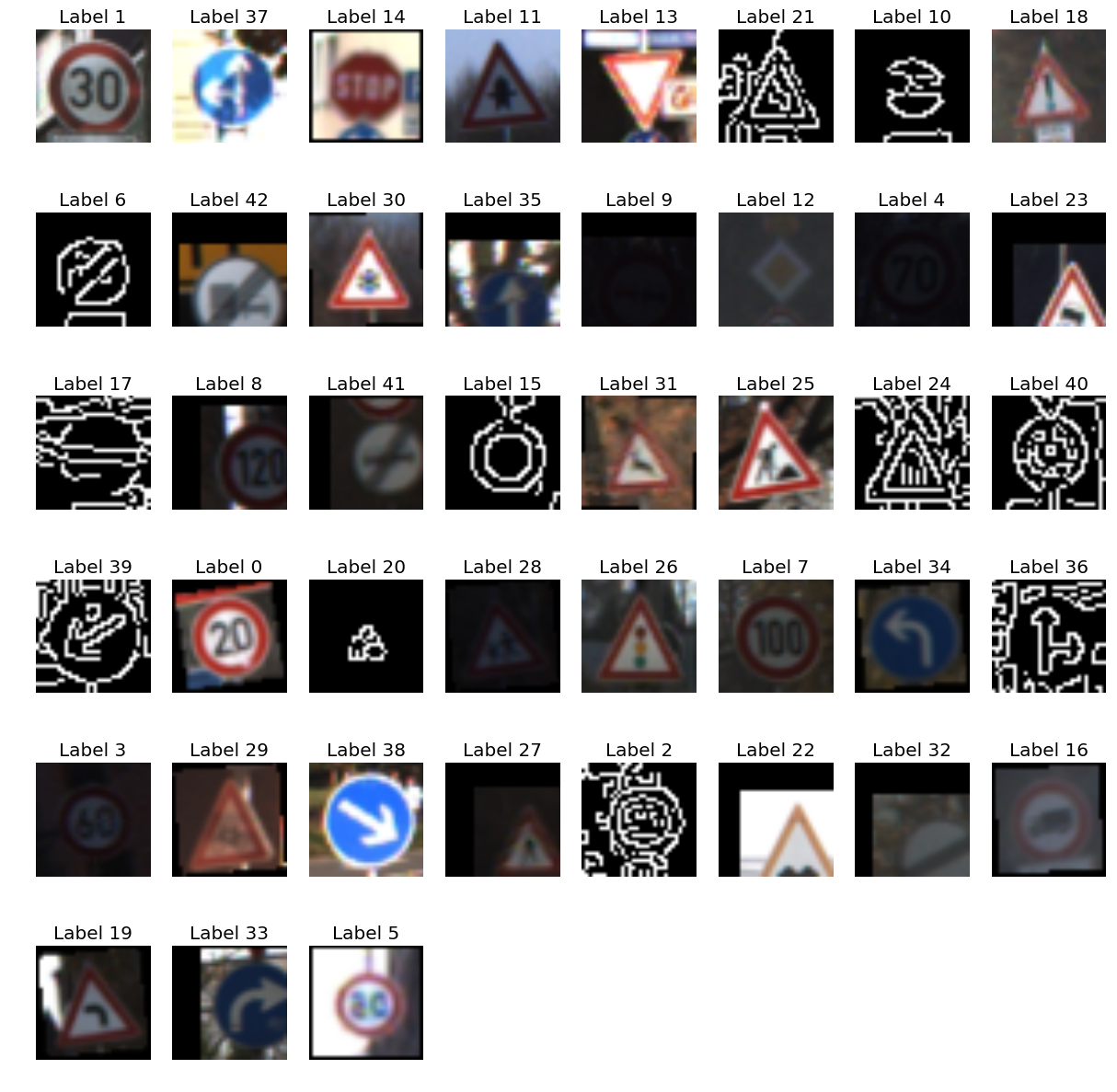
Include an exploratory visualization of the dataset
### Data exploration visualization code goes here.
### Feel free to use as many code cells as needed.
import matplotlib
import matplotlib.pyplot as plt
from mpl_toolkits.axes_grid1 import ImageGrid
from matplotlib.offsetbox import AnchoredText
from matplotlib.patheffects import withStroke
# Visualizations will be shown in the notebook.
%matplotlib inline
matplotlib.style.use('ggplot')
# Show a single image of each type of label
print(train['features'].shape, train['labels'].shape)
image_with_label = zip(train['features'], train['labels'])
seen_labels = set()

fig = plt.figure(figsize=(200, 200))
total_unique_labels = len(set(train['labels']))
unique_rows = total_unique_labels // 8 + 1

def draw_image(grid_cell, img, txt):
    im = grid[i].imshow(img)
    size = dict(size="xx-large")
    at = AnchtoredText(signname, loc=3, prop=size,
                  pad=0., borderpad=0.5,
                  frameon=False)
    grid_cell.add_artist(at)
    at.txt._text.set_path_effects([withStroke(foreground="w", linewidth=3)])

i = 1
plt.figure(figsize=(15, 15))
for i_l in image_with_label:
    img, label = i_l
    if label not in seen_labels:
        signname = get_signname(label)
        plt.subplot(unique_rows, 8, i)  # A grid of 8 rows x 8 columns
        plt.axis('off')
        plt.title("Label {0}".format(label))
        plt.imshow(img)
        seen_labels.add(label)
        i += 1

plt.show()
(172860, 32, 32, 3) (172860,)


<matplotlib.figure.Figure at 0x7ff92c37e048>
Signnames Corresponding to Integer Labels
| ClassId | SignName |
|---|---|
| 0 | Speed limit (20km/h) |
| 1 | Speed limit (30km/h) |
| 2 | Speed limit (50km/h) |
| 3 | Speed limit (60km/h) |
| 4 | Speed limit (70km/h) |
| 5 | Speed limit (80km/h) |
| 6 | End of speed limit (80km/h) |
| 7 | Speed limit (100km/h) |
| 8 | Speed limit (120km/h) |
| 9 | No passing |
| 10 | No passing for vehicles over 3.5 metric tons |
| 11 | Right-of-way at the next intersection |
| 12 | Priority road |
| 13 | Yield |
| 14 | Stop |
| 15 | No vehicles |
| 16 | Vehicles over 3.5 metric tons prohibited |
| 17 | No entry |
| 18 | General caution |
| 19 | Dangerous curve to the left |
| 20 | Dangerous curve to the right |
| 21 | Double curve |
| 22 | Bumpy road |
| 23 | Slippery road |
| 24 | Road narrows on the right |
| 25 | Road work |
| 26 | Traffic signals |
| 27 | Pedestrians |
| 28 | Children crossing |
| 29 | Bicycles crossing |
| 30 | Beware of ice/snow |
| 31 | Wild animals crossing |
| 32 | End of all speed and passing limits |
| 33 | Turn right ahead |
| 34 | Turn left ahead |
| 35 | Ahead only |
| 36 | Go straight or right |
| 37 | Go straight or left |
| 38 | Keep right |
| 39 | Keep left |
| 40 | Roundabout mandatory |
| 41 | End of no passing |
| 42 | End of no passing by vehicles over 3.5 metric … |
# Draw a histogram of how many features we have per label
bincounts = np.bincount(train['labels'])
bincounts = bincounts[train['labels']]
fig, ax = plt.subplots()
ax.bar(train['labels'], bincounts)
plt.show()
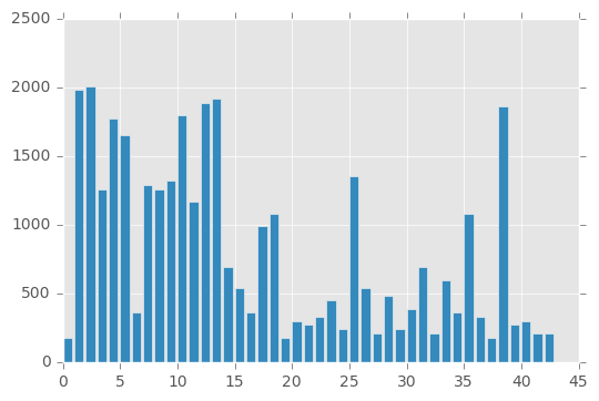
Input Data Augmentation
The input data is not balanced across the labels which could affect the accuracy of the neural net. As can be seen from the graph above, some labels have a larger amount of data than others.
So for this reason I augmented the input data so that it could provide a uniform set of training data.
There are multiple techniques which can be used to augment the data and there is even a library which can be used to augment the training data. ImgAug Link
However, I wrote my own code using a mix of opencv and skimage libraries to have a better control over the whole process. Also there were restrictions with what kinds of image augmentation could be performed which I wasn’t sure could be handled with ImgAug. Generating such a huge dataset is computationally expensive and hence I used python’s multiprocessing to speed up that process. 8 threads were launched to parallelize the operation across the 8 cores I had available on the cpu to near utilize 100% of cpu time. This brought down the time from about 20 hrs on a Macbook Pro 15” to about 7 mins on a desktop with core i7 & 32 gb memory.
Techniques for Augmentation
Techniques
Original Image:

- Random rotations between -10 and 10 degrees.

- Random translation between -10 and 10 pixels in any direction.

- Random flipping horizontally or vertically or both depending on sign. There are restrictions on this since flipping a traffic sign could change it’s meaning. Hence, labels have been classified on whether they can be flipped or not.

- Canny Edge detection


Step 2: Design and Test a Model Architecture
Pre-process the Data Set (normalization, grayscale, etc.)
Image pre-processing really didn’t help in improving the accuracy of the networks I tried. I tried a couple of techniques like
- Grayscaling
- Normalization
However, in the end I decided not to use any preprocessing but the code is capable of performing preprocessing if necessary, if deemed in the future when improving the accuracy.
### Preprocess the data here. Preprocessing steps could include normalization, converting to grayscale, etc.
### Feel free to use as many code cells as needed.
import numpy as np

import cv2
import tensorflow as tf
from tensorflow.contrib.layers import flatten

import pickle

from sklearn.model_selection import train_test_split
from sklearn.utils import shuffle
from skimage.transform import rotate
from skimage.transform import warp
from skimage.transform import ProjectiveTransform

import argparse

import pandas as pd
import random
import matplotlib
import matplotlib.pyplot as plt
from IPython.display import Image

from scipy import ndimage

import multiprocessing

matplotlib.style.use('ggplot')
Helper Functions
def print_header(txt):
    print("-" * 100)
    print(txt)
    print("-" * 100)


def print_progress_bar(iteration, total, prefix='', suffix='', decimals=1, bar_length=100):
    """
    Call in a loop to create terminal progress bar
    @params:
        iteration   - Required  : current iteration (Int)
        total       - Required  : total iterations (Int)
        prefix      - Optional  : prefix string (Str)
        suffix      - Optional  : suffix string (Str)
        decimals    - Optional  : positive number of decimals in percent complete (Int)
        bar_length  - Optional  : character length of bar (Int)
    """
    str_format = "{0:." + str(decimals) + "f}"
    percents = str_format.format(100 * (iteration / float(total)))
    filled_length = int(round(bar_length * iteration / float(total)))
    bar = '█' * filled_length + '-' * (bar_length - filled_length)

    sys.stdout.write('\r%s |%s| %s%s %s' % (prefix, bar, percents, '%', suffix)),

    if iteration == total:
        sys.stdout.write('\n')
    sys.stdout.flush()
Tensorflow Helper Functions
Helper Classes
Image Class
class Image:
    @staticmethod
    def rotate_image(img, label):
        # Rotate the image by a random angle (-45 to 45 degrees)
        # Rotation has to be done within a very narrow range since it could
        # affect the meaning of the sign itself.
        # Choosing -10 to 10 degrees
        angle = np.random.choice(np.random.uniform(-10,10,100))
        dst = ndimage.rotate(img, angle)
        height, width = img.shape[:2]
        dst = cv2.resize(dst, (width, height))
        return dst

    @staticmethod
    def translate_image(img, label):
        tx = np.random.choice(np.arange(10))
        ty = np.random.choice(np.arange(10))
        M = np.float32([[1, 0, tx], [0, 1, ty]])
        rows, cols, _ = img.shape
        dst = cv2.warpAffine(img, M, (cols, rows))
        return dst

    @staticmethod
    def flip_image(img, label):
        can_flip_horizontally = np.array([11, 12, 13, 15, 17, 18, 22, 26, 30, 35])
        # Classes of signs that, when flipped vertically, should still be classified as the same class
        can_flip_vertically = np.array([1, 5, 12, 15, 17])
        # Classes of signs that, when flipped horizontally and then vertically,
        #  should still be classified as the same class
        can_flip_both = np.array([32, 40])

        flipped = None

        if label in can_flip_horizontally:
            flipped = cv2.flip(img, 1)
        elif label in can_flip_vertically:
            flipped = cv2.flip(img, 0)
        elif label in can_flip_both:
            flipped = cv2.flip(img, np.random.choice([-1, 0, 1]))

        return flipped

    @staticmethod
    def edge_detected(img, label):
        slice = np.uint8(img)
        canny = cv2.Canny(slice, 50, 150)
        backtorgb = cv2.cvtColor(canny, cv2.COLOR_GRAY2RGB)
        return backtorgb

    @staticmethod
    def perform_random_op(img, label):
        ops = [Image.edge_detected, Image.flip_image,
               Image.translate_image, Image.rotate_image,
              ]

        random_op = ops[random.randint(0, len(ops) - 1)]
        print(str(random_op))
        new_img = random_op(img, label)
        while new_img is None:
            random_op = ops[random.randint(0, len(ops) - 1)]
            new_img = random_op(img, label)

        return new_img

    @staticmethod
    def insert_subimage(image, sub_image, y, x):
        h, w, c = sub_image.shape
        image[y:y+h, x:x+w, :]=sub_image
        return image

    @staticmethod
    def grayscale(image):
        # use lumnosity to convert to grayscale as done by GIMP software
        # refer https://www.johndcook.com/blog/2009/08/24/algorithms-convert-color-grayscale/
        image = image[:,:,0] * .21 + image[:,:,1] * .72 + image[:,:,2]* .07
        return image

    @staticmethod
    def normalize(data):
        return data / 255 * 0.8 + 0.1

    # iterate through the image set and convert them to grayscale images
    @staticmethod
    def preprocess(data):
        gray_images = []
        for image in data:
            gray = Image.grayscale(image)
            gray = np.reshape(gray,(32 , 32, 1))
            gray_images.append(gray)

        gray_images = np.array(gray_images)
        gray_images = Image.normalize(gray_images)

        return gray_images
Data Class
class Data:
    """
    Encode the different data so its easier to pass them around
    """
    def __init__(self, X_train, y_train, X_validation, y_validation, X_test,
                 y_test, images_from_internet, filenames_from_internet):
        self.X_train = X_train
        self.y_train = y_train
        self.X_validation = X_validation
        self.y_validation = y_validation
        self.X_test = X_test
        self.y_test = y_test
        self.images_from_internet = images_from_internet
        self.filenames_from_internet = filenames_from_internet

        self.frame = pd.read_csv('signnames.csv')

    def preprocess(self):
        # Normalize the RGB values to 0.0 to 1.0
        self.X_train = Image.preprocess(self.X_train)
        self.X_test  = Image.preprocess(self.X_test)
        self.X_validation = Image.preprocess(self.X_validation)

    def get_signname(self, label_id):
        return self.frame["SignName"][label_id]

    def display_statistics(self):
        """
        Figure out statistics on the data using Pandas.
        """
        _, height, width, channel = self.X_train.shape
        num_class = np.max(self.y_train) + 1

        training_data = np.concatenate((self.X_train, self.X_validation))
        training_labels = np.concatenate((self.y_train, self.y_validation))

        num_sample = 10
        results_image = 255.*np.ones(shape=(num_class*height, (num_sample + 2 + 22) * width, channel), dtype=np.float32)
        for c in range(num_class):
            indices = np.array(np.where(training_labels == c))[0]
            random_idx = np.random.choice(indices)
            label_image = training_data[random_idx]
            Image.insert_subimage(results_image, label_image, c * height, 0)

            #make mean
            idx = list(np.where(training_labels == c)[0])
            mean_image = np.average(training_data[idx], axis=0)
            Image.insert_subimage(results_image, mean_image, c * height, width)

            #make random sample
            for n in range(num_sample):
                sample_image = training_data[np.random.choice(idx)]
                Image.insert_subimage(results_image, sample_image, c*height, (2 + n) * width)

            #print summary
            count=len(idx)
            percentage = float(count)/float(len(training_data))
            cv2.putText(results_image, '%02d:%-6s'%(c, self.get_signname(c)), ((2+num_sample)*width, int((c+0.7)*height)), cv2.FONT_HERSHEY_SIMPLEX, 0.5, (0, 0, 0), 1)
            cv2.putText(results_image, '[%4d]'%(count), ((2+num_sample+14)*width, int((c+0.7)*height)),cv2.FONT_HERSHEY_SIMPLEX,0.5,(0, 0, 255), 1)
            cv2.rectangle(results_image,((2+num_sample+16)*width, c*height),((2+num_sample+16)*width + round(percentage * 3000), (c+1)*height),(0, 0, 255), -1)


        cv2.imwrite('augmented/data_summary.jpg',cv2.cvtColor(results_image, cv2.COLOR_BGR2RGB))

    def visualize_training_data(self):
        _, height, width, channel = self.X_train.shape
        num_class = np.max(self.y_train) + 1

        training_data = np.concatenate((self.X_train, self.X_validation))
        training_labels = np.concatenate((self.y_train, self.y_validation))

        for c in range(0, num_class):
            print("Class %s" % c)
            indices = np.array(np.where(training_labels == c))[0]
            total_cols = 50
            total_rows = len(indices) / total_cols + 1

            results_image = 255. * np.ones(shape=(total_rows * height, total_cols * width, channel),
                                           dtype=np.float32)
            for n in range(len(indices)):
                sample_image = training_data[indices[n]]
                Image.insert_subimage(results_image, sample_image, (n / total_cols) * height, (n % total_cols) * width)

            filename = str(c) + ".png"
            cv2.imwrite('augmented/' + filename, cv2.cvtColor(results_image, cv2.COLOR_BGR2RGB))
            print("Wrote image: %s" % filename)

    def _augment_data_for_class(self, label_id, augmented_size, training_labels, training_data):
        """
        Internal method which will augment the data size for the specified label.
        It will calculate the initial size and augment it to its size.
        """
        print("\nAugmenting class: %s" % label_id)

        # find all the indices for the label id
        indices = np.array(np.where(training_labels == label_id))[0]
        total_data_len = len(indices)

        if indices.shape == 0:
            return np.array([]), np.array([])

        print("Label %s has %s images. Augmenting by %s images to %s images" % (label_id, total_data_len, (augmented_size - total_data_len), augmented_size))

        new_training_data = []
        new_training_label = []
        # Find a random ID from the indices and perform a random operation
        for i in range(0, (augmented_size - total_data_len)):
            print_progress_bar(i, (augmented_size - total_data_len), prefix='Progress:', suffix='Complete', bar_length=50)
            random_idx = np.random.choice(indices)
            img = training_data[random_idx]
            nimg = Image.perform_random_op(img=img, label=random_idx)

            # Add this to the training dataset
            new_training_data.append(nimg)
            new_training_label.append(label_id)

        new_training_data = np.array(new_training_data)
        new_training_label = np.array(new_training_label)

        return new_training_data, new_training_label

    def augment_data(self, augmentation_factor):
        """
        Augment the input data with more data so that we can make all the labels
        uniform
        """
        # Find the class label which has the highest images. We will decide the
        # augmentation size based on that multipled by the augmentation factor
        pool = multiprocessing.Pool(multiprocessing.cpu_count())

        training_labels = np.concatenate((self.y_train, self.y_validation))
        training_data   = np.concatenate((self.X_train, self.X_validation))

        bincounts = np.bincount(training_labels)
        label_counts = bincounts.shape[0]

        max_label_count = np.max(bincounts)
        augmentation_data_size = max_label_count * augmentation_factor

        print_header("Summary for Training Data for Augmentation")
        print("Max Label Count: %s" % max_label_count)
        print("Augmented Data Size: %s" % augmentation_data_size)

        args = []
        for i in range(0, label_counts):
            if i in training_labels:
                args.append((i, augmentation_data_size, training_labels, training_data))

        results = pool.starmap(self._augment_data_for_class, args)
        pool.close()
        pool.join()

        features, labels = zip(*results)

        features = np.array(features)
        labels = np.array(labels)

        augmented_features = np.concatenate(features, axis=0)
        augmented_labels = np.concatenate(labels, axis=0)
        all_features = np.concatenate(np.array([training_data, augmented_features]), axis=0)
        all_labels = np.concatenate(np.array([training_labels, augmented_labels]), axis=0)

        all_features, all_labels = shuffle(all_features, all_labels)

        train = {}
        train['features'] = all_features
        train['labels'] = all_labels

        f = open('augmented/augmented.p', 'wb')
        pickle.dump(train, f, protocol=4)
Config Class
class NNConfig:
    """
    This class keeps all the configuration for running this network together at
    one spot so its easier to run it.
    """
    def __init__(self, EPOCHS, BATCH_SIZE, MAX_LABEL_SIZE, INPUT_LAYER_SHAPE,
                 LEARNING_RATE, SAVE_MODEL, NN_NAME, USE_AUGMENTED_FILE):
        """
        EPOCHS: How many times are we running this network
        BATCH_SIZE: How many inputs do we consider while running this data
        MAX_LABEL_SIZE: What is the maximum label size
                        (For example we have 10 classes for MNIST so its 10
                        For Traffic Database its 43)
        INPUT_LAYER_SHAPE: What is the shape of the input image.
                           How many channels does it have.
                           Eg. MNIST: 28x28x1
                           Traffic Sign: 32x32x3
        LEARNING_RATE: Learning rate for the network
        """
        self.EPOCHS = EPOCHS
        self.BATCH_SIZE = BATCH_SIZE
        self.MAX_LABELS = MAX_LABEL_SIZE
        self.INPUT_LAYER_SHAPE = INPUT_LAYER_SHAPE
        self.LEARNING_RATE = LEARNING_RATE
        self.SAVE_MODEL = SAVE_MODEL
        self.NN_NAME = NN_NAME
        self.IS_TRAINING = False
        self.USE_AUGMENTED_FILE = USE_AUGMENTED_FILE

        assert(len(INPUT_LAYER_SHAPE) == 3)

        self.NUM_CHANNELS_IN_IMAGE = INPUT_LAYER_SHAPE[2]
Tensor Ops Class
class TensorOps:
    """
    This class stores the tensor ops which will be used in training, testing and prediction
    """
    def __init__(self, x, y, dropout_keep_prob, training_op, accuracy_op, loss_op, logits, saver):
        """
        x: Tensor for the input class
        y: Tensor for the output class
        training_op: Training operation Tensor
        accuracy_op: Tensor for the accuracy operation
        saver: Used for saving the eventual model
        """
        self.x = x
        self.y = y
        self.dropout_keep_prob = dropout_keep_prob
        self.training_op = training_op
        self.accuracy_op = accuracy_op
        self.loss_op = loss_op
        self.logits = logits
        self.saver = saver
Tensorflow Helper Functions
def convolutional_layer(input, num_input_filters, num_output_filters, filter_shape,
                        strides, padding, mean, stddev, activation_func=None, name=""):
    conv_W = tf.Variable(tf.truncated_normal(shape=filter_shape+(num_input_filters, num_output_filters), mean=mean, stddev=stddev), name+"_weights")
    conv_b = tf.Variable(tf.zeros(num_output_filters), name=name+"_bias")

    conv = tf.nn.conv2d(input, conv_W, strides, padding) + conv_b

    # Activation Layer
    if activation_func is not None:
        conv = activation_func(conv)

    print(name + ": " + str(conv.get_shape().as_list()))
    return conv, num_output_filters


def fully_connected_layer(input, input_size, output_size, mean, stddev,
                          activation_func, dropout_prob, name):
    fc_W = tf.Variable(tf.truncated_normal(shape=(input_size, output_size),
                       mean=mean, stddev=stddev), name=name + "_W")
    fc_b = tf.Variable(tf.zeros(output_size), name=name + "_b")
    fc   = tf.matmul(input, fc_W) + fc_b

    if activation_func is not None:
        fc = activation_func(fc, name=name + "_relu")

    fc = tf.nn.dropout(fc, dropout_prob)

    return fc, output_size


def maxpool2d(input, ksize, strides, padding, name=""):
    maxpool = tf.nn.max_pool(input, ksize, strides, padding, name=name)

    return maxpool

def flatten_layer(layer):
    # Get the shape of the input layer.
    layer_shape = layer.get_shape()
    num_features = layer_shape[1:4].num_elements()
    layer_flat = tf.reshape(layer, [-1, num_features])
    return layer_flat, num_features
Model Architecture
Why choose Convolutional Networks
Traditional neural networks take the approach of mapping individual outputs to neurons, thereby completely ignoring the spatial structure and relationship the inputs might have with each other. For instance, it treats input pixels which are far apart and close together on exactly the same footing. Images fall into the category of input where the pixels used for identifying objects are often have a relation to each other. CNN’s are a special group of Neural Networks which use filters in their initial layers to extract spatial information. Filters are a traditional concept from Image Processing and Computer Vision. Filters are used to extract edges, blur out images, sharpen images so on and so forth. Thus filters are the magic that extract the spatial information hidden in images.
Why Multilayer CNN’s
Multilayer CNN’s are therefore suited to this kind of image identification problem. The reason for this is that in multilayer CNN’s, multiple filters of different sizes are used to identify the various features which can be extracted from an image. For example when identifying a dog’s face, different size filters can extract different features from the face like eyes, nose, jaws etc.
For the purpose of this project I tried out 5 different networks with various parameters and combinations. The 5 networks are as follows.
- Simple Neural Network with 1 Convolution Layer (Simple NN1)
- Simple Neural Network with 2 Convolution Layer (Simple NN2)
- LeNet
- DeepNet: A Deep network with merging between multiple convolution layers
- DeepNetNoMerging: A Deep network with no merging between multiple convolution layers.
Overall, I found that training data augmentation did not play any major role in improving the accuracy. As can be seen the networks are of varying complexity. They vary from a really simple network to extremely complex networks. However, since the image size is small, even a simple network can perform almost similar to a relative complex network.
Parameter Tuning
Most of the parameter tuning was done by trial and error. Some parameters worked well while some didn’t and hence weren’t included as a part of the network.
- Batch Normalization: Batch normalization actually reduced the accuracy when introduced in fully connected layers. Hence didn’t include that.
- L2 Loss: L2 Loss calculation was added to the loss function which improved the accuracy of networks like Lenet by about 2 to 3%
- Dropouts: Dropouts helped mainly in the complex networks like DeepNet variations but not in the simpler networks. Infact for simpler network the dropout was always kept at 1.0.
- Batch Size: I chose a batch size of 128 since that meant that we don’t have to keep a huge amount of memory blocked up. Since I was running the network on a GTX 1080 as well as CPU it was important to make sure that I do exceed the amount of memory required for the data as well as for the Deep Networks. 128 seemed to work well in this case.
- Epoch Size: Epoch size was decided based on 2 factors. Convergance rate and speed of convergance. I ran multiple models with various parameters on multiple machines on both CPU (with SSE & AVX) & Gtx 1080. Finally after observing I noticed that an epoch between 75 to 150 seemed to work well and a decent convergance rate was achieved.
Adam Optimizer
I chose the Adam Optimizer over the Gradient Descent Optimizer since it provided faster convergance than SGD in this case.
Choosing a Network
The reason I chose to try out 5 different networks is because of the fact that I wanted to see how different models perform on such a dataset. Speed, Accuracy and memory were all important factors. In the testing phase, the biggest issue was speed and the feedback loop because of this slowness. I initially tried out complex models before realizing that it wasn’t scalable on the CPU. Hence I started working on simpler networks so that they could converge faster and based on the accuracy I saw it could be a reasonable model to try out first before approaching complex models.
Simple NN1

def simple_1conv_layer_nn(x, dropout_keep_prob, cfg):
    mu = 0
    sigma = 0.1

    # Convolutional Layer 1: Input 32x32x3         Output = 26x26x12
    conv1, num_output_filters = convolutional_layer(x, num_input_filters=cfg.NUM_CHANNELS_IN_IMAGE, num_output_filters=12,
                                                    filter_shape=(7, 7), strides=[1,1,1,1], padding='VALID',
                                                    mean=mu, stddev=sigma, activation_func=tf.nn.relu, name="conv2d_1")

    # Now use a fully connected Layer
    fc0 = flatten(conv1)

    shape = fc0.get_shape().as_list()[1]

    # Use 2 more layers
    # Fully Connected: Input = 192               Output = 96
    fc1, output_size = fully_connected_layer(fc0, shape, 96, mu, sigma, tf.nn.relu, dropout_keep_prob, name="fc1")

    # Fully Connected: Input = 96               Output = 43
    logits, output_size = fully_connected_layer(fc1, output_size, cfg.MAX_LABELS, mu, sigma,
                                                activation_func=None, dropout_prob=1.0, name="logits")

    # Create a Network param dict for visualization
    network_params = {
        "conv1": conv1,
        "fc0": fc0,
        "fc1": fc1,
        "logits": logits
    }

    cfg.NETWORK_PARAMS = network_params

    return logits
Simple NN2

def simple_2conv_layer_nn(x, dropout_keep_prob, cfg):
    mu = 0
    sigma = 0.1

    # Convolutional Layer 1: Input 32x32x3         Output = 26x26x12
    conv1, num_output_filters = convolutional_layer(x, num_input_filters=cfg.NUM_CHANNELS_IN_IMAGE, num_output_filters=12,
                                                    filter_shape=(5, 5), strides=[1,1,1,1], padding='SAME',
                                                    mean=mu, stddev=sigma, activation_func=tf.nn.relu, name="conv2d_1")

    maxpool1 = maxpool2d(conv1, ksize=[1, 2, 2, 1], strides=[1, 2, 2, 1], padding='VALID', name="maxpool1")


    conv2, num_output_filters = convolutional_layer(maxpool1, num_input_filters=num_output_filters, num_output_filters=num_output_filters * 2,
                                                    filter_shape=(7, 7), strides=[1,1,1,1], padding='SAME',
                                                    mean=mu, stddev=sigma, activation_func=tf.nn.relu, name="conv2d_1")

    maxpool2 = maxpool2d(conv2, ksize=[1, 2, 2, 1], strides=[1, 2, 2, 1], padding='VALID', name="maxpool2")

    # Now use a fully connected Layer
    fc0 = flatten(maxpool2)

    shape = fc0.get_shape().as_list()[1]

    # Use 2 more layers
    # Fully Connected: Input = 192               Output = 96
    fc1, output_size = fully_connected_layer(fc0, shape, 96, mu, sigma,
                                             activation_func=tf.nn.relu, dropout_prob=dropout_keep_prob, name="fc1")

    # Fully Connected: Input = 96               Output = 43
    logits, output_size = fully_connected_layer(fc1, 96, 43, mu, sigma,
                                                activation_func=None, dropout_prob=1.0, name="logits")

    # Create a Network param dict for visualization
    network_params = {
        "conv1": conv1,
        "conv2": conv2,
        "fc0": fc0,
        "fc1": fc1,
        "logits": logits
    }

    cfg.NETWORK_PARAMS = network_params

    return logits
Deep Network Implementation
DeepNetMergeLayers
The deep net merge layer network has essentially 4 major groups with each group consisting of multiple layers. It starts with a 1x1 layer which is intended to reduce the image brightness effects. The rest of the layers are documented in the table below.
| Layer | Description |
|---|---|
| Input | 32x32x3 RGB image |
| Convolution 1x1 | 1x1 stride, SAME Padding, 3 output filters |
| Convolution 5x5 | 1x1 stride, SAME padding, 8 output Filters |
| RELU | |
| Convolution 5x5 | 1x1 stride, SAME padding, 8 output Filters |
| RELU | |
| Maxpool | 2x2 size kernel, 2x2 stride, |
| Dropout 1 | |
| Convolution 5x5 | 1x1 stride, SAME padding, 16 output Filters |
| RELU | |
| Convolution 5x5 | 1x1 stride, SAME padding, 16 output Filters |
| RELU | |
| Maxpool | 2x2 size kernel, 2x2 stride, |
| Dropout 2 | |
| Convolution 5x5 | 1x1 stride, SAME padding, 32 output Filters |
| RELU | |
| Convolution 5x5 | 1x1 stride, SAME padding, 32 output Filters |
| RELU | |
| Maxpool | 2x2 size kernel, 2x2 stride, |
| Dropout 3 | |
| Flatten | Dropout1, Dropout2, Dropout3 |
| Fully connected | 1024 Outputs |
| Fully connected | 1024 Outputs |
| Logits Softmax | 43 Outputs |

def DeepNetMergeLayers(x, dropout_keep_prob, cfg):
    mu = 0
    sigma = 0.1

    conv1, num_output_filters = convolutional_layer(x, num_input_filters=cfg.NUM_CHANNELS_IN_IMAGE, num_output_filters=3,
                                                    filter_shape=(1, 1), strides=[1,1,1,1], padding='SAME',
                                                    mean=mu, stddev=sigma, activation_func=tf.nn.relu, name="conv2d_1")


    # Group 1
    conv2, num_output_filters = convolutional_layer(conv1, num_input_filters=num_output_filters, num_output_filters=8,
                                                    filter_shape=(5, 5), strides=[1,1,1,1], padding='SAME',
                                                    mean=mu, stddev=sigma, activation_func=tf.nn.relu, name="conv2d_2")

    conv3, num_output_filters = convolutional_layer(conv2, num_input_filters=num_output_filters, num_output_filters=8,
                                                    filter_shape=(5, 5), strides=[1,1,1,1], padding='SAME',
                                                    mean=mu, stddev=sigma, activation_func=tf.nn.relu, name="conv2d_3")

    maxpool1 = maxpool2d(conv3, ksize=[1, 2, 2, 1], strides=[1, 2, 2, 1], padding='SAME', name="maxpool1")

    dropout1 = tf.nn.dropout(maxpool1, dropout_keep_prob, name="dropout1")

    # Group 2
    conv4, num_output_filters = convolutional_layer(dropout1, num_input_filters=num_output_filters, num_output_filters=16,
                                                    filter_shape=(5, 5), strides=[1,1,1,1], padding='SAME',
                                                    mean=mu, stddev=sigma, activation_func=tf.nn.relu, name="conv2d_4")

    conv5, num_output_filters = convolutional_layer(conv4, num_input_filters=num_output_filters, num_output_filters=16,
                                                    filter_shape=(5, 5), strides=[1,1,1,1], padding='SAME',
                                                    mean=mu, stddev=sigma, activation_func=tf.nn.relu, name="conv2d_5")

    maxpool2 = maxpool2d(conv5, ksize=[1, 2, 2, 1], strides=[1, 2, 2, 1], padding='SAME', name="maxpool2")

    dropout2 = tf.nn.dropout(maxpool2, dropout_keep_prob, name="dropout2")

    # Group 3
    conv6, num_output_filters = convolutional_layer(dropout2, num_input_filters=num_output_filters, num_output_filters=32,
                                                    filter_shape=(5, 5), strides=[1,1,1,1], padding='SAME',
                                                    mean=mu, stddev=sigma, activation_func=tf.nn.relu, name="conv2d_6")

    conv7, num_output_filters = convolutional_layer(conv6, num_input_filters=num_output_filters, num_output_filters=32,
                                                    filter_shape=(5, 5), strides=[1,1,1,1], padding='SAME',
                                                    mean=mu, stddev=sigma, activation_func=tf.nn.relu, name="conv2d_6")

    maxpool3 = maxpool2d(conv7, ksize=[1, 2, 2, 1], strides=[1, 2, 2, 1], padding='SAME', name="maxpool3")

    dropout3 = tf.nn.dropout(maxpool3, dropout_keep_prob, name="dropout3")

    # Now Flatten all the layers together
    layer_flat_group1, num_fc_layers_group1 = flatten_layer(dropout1)
    layer_flat_group2, num_fc_layers_group2 = flatten_layer(dropout2)
    layer_flat_group3, num_fc_layers_group3 = flatten_layer(dropout3)
    layer_flat = tf.concat(values=[layer_flat_group1, layer_flat_group2, layer_flat_group3], axis=1)

    num_fc_layers = num_fc_layers_group1 + num_fc_layers_group2 + num_fc_layers_group3

    fc_size1 = 1024
    ## FC_size
    fc_size2 = 1024

    # Fully Connected: Input = 1024               Output = 1024
    fc1, output_size = fully_connected_layer(layer_flat, num_fc_layers, num_fc_layers, mu, sigma,
                                             activation_func=tf.nn.relu, dropout_prob=dropout_keep_prob, name="fc1")

    fc2, output_size = fully_connected_layer(fc1, num_fc_layers, num_fc_layers, mu, sigma,
                                             activation_func=tf.nn.relu, dropout_prob=dropout_keep_prob, name="fc2")

    # Fully Connected: Input = 96               Output = 43
    logits, _ = fully_connected_layer(fc1, num_fc_layers, cfg.MAX_LABELS, mu, sigma,
                                      activation_func=None, dropout_prob=1.0, name="logits")

    return logits
Deep Network - No Merge Layers
The deep net merge layer network has essentially 4 major groups with each group consisting of multiple layers. It starts with a 1x1 layer which is intended to reduce the image brightness effects. The rest of the layers are documented in the table below.
| Layer | Description |
|---|---|
| Input | 32x32x3 RGB image |
| Convolution 1x1 | 1x1 stride, SAME Padding, 3 output filters |
| Convolution 3x3 | 1x1 stride, SAME padding, 12 output Filters |
| RELU | |
| Convolution 5x5 | 1x1 stride, VALID padding, Outputs 28x28x24, 24 output Filters |
| RELU | |
| Convolution 5x5 | 1x1 stride, VALID padding, Outputs 24x24x48, 48 output Filters |
| RELU | |
| Convolution 9x9 | 1x1 stride, SAME padding, Outputs 16x16x96, 96 output Filters |
| RELU | |
| Convolution 3x3 | 1x1 stride, SAME padding, Outputs 16x16x192, 192 output Filters |
| RELU | |
| Maxpool | 2x2 maxpool, 2x2 stride, SAME, Outputs 16x16x384 |
| Convolution 11x11 | 1x1 stride, SAME padding, Outputs 8x8x384, 384 output Filters |
| RELU | |
| Maxpool | 2x2 maxpool, 2x2 stride, SAME, Outputs 4x4x384 |
| Flatten | 6144 Outputs |
| Fully connected | 3072 Outputs |
| Fully connected | 1536 Outputs |
| Fully connected | 768 Outputs |
| Fully connected | 384 Outputs |
| Fully connected | 192 Outputs |
| Fully connected | 96 Outputs |
| Logits Softmax | 43 Outputs |

def DeepNet(x, dropout_keep_prob, cfg):
    # Hyper parameters
    mu = 0
    sigma = 0.1

    one_by_one, num_output_filters = convolutional_layer(x, num_input_filters=cfg.NUM_CHANNELS_IN_IMAGE, num_output_filters=3,
                                                        filter_shape=(1, 1), strides=[1,1,1,1], padding='SAME',
                                                        mean=mu, stddev=sigma, activation_func=tf.nn.relu, name="conv2d_1")

    # Convolutional Layer 1: Input 32x32x3         Output = 32x32x12
    conv1, num_output_filters = convolutional_layer(one_by_one, num_input_filters=3, num_output_filters=12,
                                                    filter_shape=(3, 3), strides=[1,1,1,1], padding='SAME',
                                                    mean=mu, stddev=sigma, activation_func=tf.nn.relu, name="conv2d_1")

    # Convolutional Layer 2: Input 32x32x12         Output = 28x28x24
    conv2, num_output_filters = convolutional_layer(conv1, num_input_filters=num_output_filters, num_output_filters=num_output_filters * 2,
                                                    filter_shape=(5, 5), strides=[1,1,1,1], padding='VALID',
                                                    mean=mu, stddev=sigma, activation_func=tf.nn.relu, name="conv2d_2")

    # Convolutional Layer 3: Input 28x28x24         Output = 24x24x48
    conv3, num_output_filters = convolutional_layer(conv2, num_input_filters=num_output_filters, num_output_filters=num_output_filters * 2,
                                                    filter_shape=(5, 5), strides=[1,1,1,1], padding='VALID',
                                                    mean=mu, stddev=sigma, activation_func=tf.nn.relu, name="conv2d_3")

    # Convolutional Layer 4: Input 24x24x48         Output = 16x16x96
    conv4, num_output_filters = convolutional_layer(conv3, num_input_filters=num_output_filters, num_output_filters=num_output_filters * 2,
                                                    filter_shape=(9, 9), strides=[1,1,1,1], padding='VALID',
                                                    mean=mu, stddev=sigma, activation_func=tf.nn.relu, name="conv2d_4")

    # Now lets add Convolutional Layers with downsampling
    conv5, num_output_filters = convolutional_layer(conv4, num_input_filters=num_output_filters, num_output_filters=num_output_filters * 2,
                                                    filter_shape=(3, 3), strides=[1,1,1,1], padding='SAME',
                                                    mean=mu, stddev=sigma, activation_func=tf.nn.relu, name="conv2d_5")

    # MaxPool Layer: Input 16x16x192                 Output = 16x16x384
    maxpool1 = tf.nn.max_pool(conv5, ksize=[1, 2, 2, 1], strides=[1, 2, 2, 1], padding='SAME', name="maxpool1")

    # Convolutional Layer 6: Input 16x16x384         Output = 8x8x384
    conv6, num_output_filters = convolutional_layer(maxpool1, num_input_filters=num_output_filters, num_output_filters=num_output_filters * 2,
                                                    filter_shape=(11, 11), strides=[1,1,1,1], padding='SAME',
                                                    mean=mu, stddev=sigma, activation_func=tf.nn.relu, name="conv2d_6")

    # MaxPool Layer: Input 8x8x384                 Output = 4x4x384
    maxpool2 = tf.nn.max_pool(conv6, ksize=[1, 2, 2, 1], strides=[1, 2, 2, 1], padding='SAME', name="maxpool2")

    # Fully Connected Layer
    fc0 = flatten(maxpool2)

    # Fully Connected: Input = 6144                Output = 3072
    fc1, output_size = fully_connected_layer(fc0, 6144, 3072, mu, sigma, tf.nn.relu, dropout_keep_prob, name="fc1")

    # Fully Connected: Input = 3072                Output = 1536
    fc2, output_size = fully_connected_layer(fc1, 3072, 1536, mu, sigma, tf.nn.relu, dropout_keep_prob, name="fc2")

    # Fully Connected: Input = 1536               Output = 768
    fc3, output_size = fully_connected_layer(fc2, 1536, 768, mu, sigma, tf.nn.relu, dropout_keep_prob, name="fc3")


    # Fully Connected: Input = 768               Output = 384
    fc4, output_size = fully_connected_layer(fc3, 768, 384, mu, sigma, tf.nn.relu, dropout_keep_prob, name="fc4")

    # Fully Connected: Input = 384               Output = 192
    fc5, output_size = fully_connected_layer(fc4, 384, 192, mu, sigma, tf.nn.relu, dropout_keep_prob, name="fc5")

    # Fully Connected: Input = 192               Output = 96
    fc6, output_size = fully_connected_layer(fc5, 192, 96, mu, sigma, tf.nn.relu, dropout_keep_prob, name="fc6")

    # Fully Connected: Input = 96               Output = 43
    # logits, output_size = fully_connected_layer(fc6, 96, 43, mu, sigma, tf.nn.relu, dropout_keep_prob, name="logits")
    logits, output_size = fully_connected_layer(fc6, 96, cfg.MAX_LABELS, mu, sigma,
                                                activation_func=None, dropout_prob=1.0, name="logits")
    return logits
LeNet
def LeNet(x, dropout_keep_prob, cfg):
    mu = 0
    sigma = 0.1

    # Convolutional Layer 1: Input 32x32x3         Output = 28x28x6
    conv1, num_output_filters = convolutional_layer(x, num_input_filters=cfg.NUM_CHANNELS_IN_IMAGE, num_output_filters=6,
                                                    filter_shape=(5, 5), strides=[1,1,1,1], padding='VALID',
                                                    mean=mu, stddev=sigma, activation_func=tf.nn.relu, name="conv2d_1")

    # Maxpool Layer : Input 28x28x6                Output = 14x14x6
    maxpool1 = maxpool2d(conv1, ksize=[1, 2, 2, 1], strides=[1, 2, 2, 1], padding='VALID', name="maxpool1")

    # Convolutional Layer : Input 14x14x6          Output = 10x10x16
    conv2, num_output_filters = convolutional_layer(maxpool1, num_input_filters=num_output_filters, num_output_filters=16,
                                                    filter_shape=(5, 5), strides=[1,1,1,1], padding='VALID',
                                                    mean=mu, stddev=sigma, activation_func=tf.nn.relu, name="conv2d_2")

    # Maxpool Layer : Input = 10x10x16             Output = 5x5x16
    maxpool2 = maxpool2d(conv2, ksize=[1, 2, 2, 1], strides=[1, 2, 2, 1], padding='VALID', name="maxpool2")

    # Fully Connected Layer
    fc0 = flatten(maxpool2)

    shape = fc0.get_shape().as_list()[1]

    # Layer 3: Fully Connected: Input = 400           Output = 120
    fc1, shape = fully_connected_layer(fc0, shape, 120, mu, sigma, tf.nn.relu, dropout_keep_prob, name="fc1")

    # Layer 4: Fully Connected: Input = 120           Output = 84
    fc2, shape = fully_connected_layer(fc1, shape, 84, mu, sigma, tf.nn.relu, dropout_keep_prob, name="fc2")

    # logits
    # MAKE SURE LOGITS HAS NO DROPOUT
    logits, _ = fully_connected_layer(fc2, shape, cfg.MAX_LABELS, mu, sigma,
                                      activation_func=None, dropout_prob=1.0,
                                      name="logits")

    # Create a Network param dict for visualization
    network_params = {
        "conv1": conv1,
        "maxpool1": maxpool1,
        "conv2": conv2,
        "maxpool2": maxpool2,
        "fc0": fc0,
        "fc1": fc1,
        "fc2": fc2,
        "logits": logits
    }

    cfg.NETWORK_PARAMS = network_params

    return logits
Lenet Original Code from Udacity
Using this only for viewing the activations
def LeNet_Udacity(x, dropout_keep_prob, cfg):
    # Arguments used for tf.truncated_normal, randomly defines variables for the weights and biases for each layer
    mu = 0
    sigma = 0.1

    # SOLUTION: Layer 1: Convolutional. Input = 32x32x3. Output = 28x28x6.
    conv1_W = tf.Variable(tf.truncated_normal(shape=(5, 5, 3, 6), mean = mu, stddev = sigma))
    conv1_b = tf.Variable(tf.zeros(6))
    conv1   = tf.nn.conv2d(x, conv1_W, strides=[1, 1, 1, 1], padding='VALID') + conv1_b

    # SOLUTION: Activation.
    conv1 = tf.nn.relu(conv1)

    # SOLUTION: Pooling. Input = 28x28x6. Output = 14x14x6.
    conv1 = tf.nn.max_pool(conv1, ksize=[1, 2, 2, 1], strides=[1, 2, 2, 1], padding='VALID')

    # SOLUTION: Layer 2: Convolutional. Output = 10x10x16.
    conv2_W = tf.Variable(tf.truncated_normal(shape=(5, 5, 6, 16), mean = mu, stddev = sigma))
    conv2_b = tf.Variable(tf.zeros(16))
    conv2   = tf.nn.conv2d(conv1, conv2_W, strides=[1, 1, 1, 1], padding='VALID') + conv2_b

    # SOLUTION: Activation.
    relu = tf.nn.relu(conv2)

    # SOLUTION: Pooling. Input = 10x10x16. Output = 5x5x16.
    maxpool1 = tf.nn.max_pool(relu, ksize=[1, 2, 2, 1], strides=[1, 2, 2, 1], padding='VALID')

    # SOLUTION: Flatten. Input = 5x5x16. Output = 400.
    fc0   = flatten(maxpool1)

    # SOLUTION: Layer 3: Fully Connected. Input = 400. Output = 120.
    fc1_W = tf.Variable(tf.truncated_normal(shape=(400, 120), mean = mu, stddev = sigma))
    fc1_b = tf.Variable(tf.zeros(120))
    fc1   = tf.matmul(fc0, fc1_W) + fc1_b

    # SOLUTION: Activation.
    fc1    = tf.nn.relu(fc1)

    # SOLUTION: Layer 4: Fully Connected. Input = 120. Output = 84.
    fc2_W  = tf.Variable(tf.truncated_normal(shape=(120, 84), mean = mu, stddev = sigma))
    fc2_b  = tf.Variable(tf.zeros(84))
    fc2    = tf.matmul(fc1, fc2_W) + fc2_b

    # SOLUTION: Activation.
    fc2    = tf.nn.relu(fc2)

    # SOLUTION: Layer 5: Fully Connected. Input = 84. Output = 10.
    fc3_W  = tf.Variable(tf.truncated_normal(shape=(84, 43), mean = mu, stddev = sigma))
    fc3_b  = tf.Variable(tf.zeros(43))
    logits = tf.matmul(fc2, fc3_W) + fc3_b

     # Create a Network param dict for visualization
    network_params = {
        "conv1": conv1,
        "conv2": conv2,
        "fc0": fc0,
        "fc1": fc1,
        "fc2": fc2,
        "logits": logits
    }

    cfg.NETWORK_PARAMS = network_params

    return logits
Train, Validate and Test the Model
A validation set can be used to assess how well the model is performing. A low accuracy on the training and validation sets imply underfitting. A high accuracy on the training set but low accuracy on the validation set implies overfitting.
Training Function
def train(cfg):
    print_header("Training " + cfg.NN_NAME + " --> Use Augmented Data: " + str(cfg.USE_AUGMENTED_FILE))
    cfg.IS_TRAINING = True
    global NETWORKS

    x = tf.placeholder(tf.float32, (None,) + cfg.INPUT_LAYER_SHAPE, name='X')
    y = tf.placeholder(tf.int32, (None), name='Y')
    dropout_keep_prob = tf.placeholder(tf.float32, name="dropout_keep_prob")

    one_hot_y = tf.one_hot(y, cfg.MAX_LABELS)

    logits = NETWORKS[cfg.NN_NAME](x, dropout_keep_prob, cfg)

    cross_entropy = tf.nn.softmax_cross_entropy_with_logits(
                    logits=logits, labels=one_hot_y)

    vars   = tf.trainable_variables()
    lossL2 = tf.add_n([ tf.nn.l2_loss(v) for v in vars
                    if 'bias' not in v.name ]) * 0.001

    loss_operation = tf.reduce_mean(cross_entropy) + lossL2

    optimizer = tf.train.AdamOptimizer(learning_rate=cfg.LEARNING_RATE)
    training_op = optimizer.minimize(loss_operation)

    correct_prediction = tf.equal(
        tf.argmax(logits, 1), tf.argmax(one_hot_y, 1))

    accuracy_op = tf.reduce_mean(tf.cast(correct_prediction, tf.float32))
    saver = tf.train.Saver(), training_op, accuracy_op

    tensor_ops = TensorOps(x, y, dropout_keep_prob, training_op, accuracy_op, loss_operation, logits, saver)
    return tensor_ops
Evaluation Function
def evaluate(sess, X_data, y_data, tensor_ops, cfg):
    cfg.IS_TRAINING = False
    num_examples = len(X_data)
    total_accuracy = 0
    for offset in range(0, num_examples, cfg.BATCH_SIZE):
        batch_x = X_data[offset: offset + cfg.BATCH_SIZE]
        batch_y = y_data[offset: offset + cfg.BATCH_SIZE]

        accuracy, loss = sess.run([tensor_ops.accuracy_op, tensor_ops.loss_op],
                            feed_dict={tensor_ops.x: batch_x, tensor_ops.y: batch_y,
                                       tensor_ops.dropout_keep_prob: 1.0})

        total_accuracy += (accuracy * len(batch_x))

    return total_accuracy / num_examples, loss
# Data Loading and processing part
from os import listdir
from os.path import isfile, join
def load_traffic_sign_data(training_file, testing_file, preprocess):
with open(training_file, mode='rb') as f:
train = pickle.load(f)
with open(testing_file, mode='rb') as f:
test = pickle.load(f)
X_train, y_train = train['features'], train['labels']
X_test, y_test = test['features'], test['labels']
# Split the data into the training and validation steps.
X_train, X_validation, y_train, y_validation = train_test_split(X_train, y_train, test_size=0.2, random_state=0)
internet_test_set_path = 'internet_test_set'
files_from_internet = [join(internet_test_set_path, f) for f in listdir(internet_test_set_path) if isfile(join(internet_test_set_path, f))]
imgs_from_internet = []
for f in files_from_internet:
img = cv2.cvtColor(cv2.imread(f), cv2.COLOR_BGR2RGB)
if img.shape != (32, 32, 3):
img = cv2.resize(img, (32, 32), interpolation = cv2.INTER_CUBIC)
imgs_from_internet.append(img)
imgs_from_internet = np.array(imgs_from_internet)
if preprocess:
X_train = Image.preprocess(X_train)
X_test = Image.preprocess(X_test)
X_validation = Image.preprocess(X_validation)
imgs_from_internet = Image.preprocess(imgs_from_internet)
data = Data(X_train, y_train, X_validation, y_validation, X_test, y_test, imgs_from_internet, files_from_internet)
return data
# Networks
NETWORKS = {
"simple_nn1": simple_1conv_layer_nn,
"simple_nn2": simple_2conv_layer_nn,
"lenet": LeNet,
"lenet_udacity": LeNet_Udacity,
"deepnetmergelayers": DeepNetMergeLayers,
"deepnet": DeepNet
}
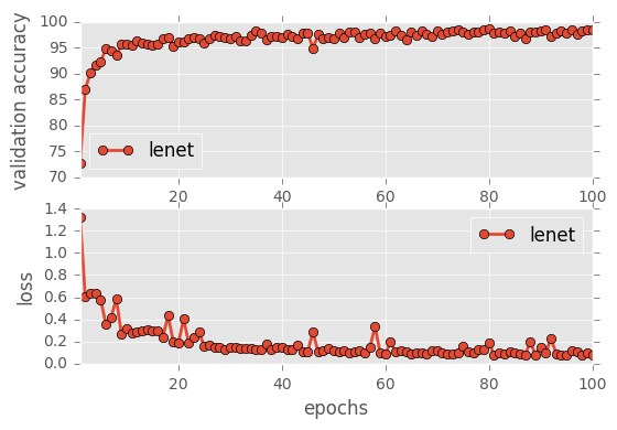
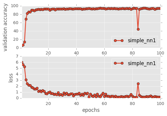
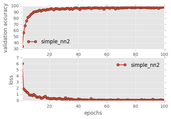
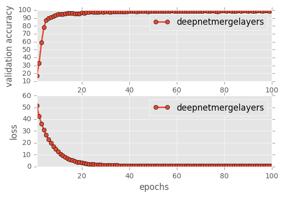
def visualize_data(df):
"""
Takes in a Pandas Dataframe and then slices and dices it to create graphs
"""
fig, (ax1, ax2) = plt.subplots(nrows = 2, ncols = 1)
ax1.set_xlabel('epochs')
ax1.set_ylabel('validation accuracy')
ax2.set_xlabel('epochs')
ax2.set_ylabel('loss')
legend1 = ax1.legend(loc='upper center', shadow=True)
legend2 = ax2.legend(loc='upper center', shadow=True)
for i, group in df.groupby('network name'):
group.plot(x='epochs', y='validation accuracy', ax=ax1, label=i, marker='o', linewidth=2)
group.plot(x='epochs', y='loss', ax=ax2, label=i, marker='o', linewidth=2)
plt.show()
def train_and_test(preprocess=False, epochs=100, learning_rate=0.001, network="lenet", batch_size=128, use_augmented_file=False, dropout_keep_prob=1.0):
global NETWORKS
if use_augmented_file:
data = load_traffic_sign_data('augmented/augmented.p', 'data/test.p', preprocess)
else:
data = load_traffic_sign_data('data/train.p', 'data/test.p', preprocess)
# Find the Max Classified Id - For example, in MNIST data we have digits
# from 0,..,9
# Hence the max classified ID is 10
# For the traffic sign database, the id's are encoded and max value is 42.
# Hence the max classified ID is 43
max_classified_id = np.max(data.y_train) + 1
print("Max Classified id: %s" % (max_classified_id))
# data.normalize_data()
dataframes = []
df = pd.DataFrame(columns=('network name', 'epochs', 'validation accuracy', 'loss'))
# Define the EPOCHS & BATCH_SIZE
cfg = NNConfig(EPOCHS=epochs,
BATCH_SIZE=batch_size,
MAX_LABEL_SIZE=max_classified_id,
INPUT_LAYER_SHAPE=data.X_train[0].shape,
LEARNING_RATE=learning_rate,
SAVE_MODEL=False,
NN_NAME=network,
USE_AUGMENTED_FILE=use_augmented_file)
tensor_ops = train(cfg)
sess = tf.Session()
sess.run(tf.global_variables_initializer())
print(dropout_keep_prob)
print("Training...\n")
for i in range(cfg.EPOCHS):
X_train, y_train = shuffle(data.X_train, data.y_train)
for offset in range(0, len(X_train), cfg.BATCH_SIZE):
end = offset + cfg.BATCH_SIZE
batch_x, batch_y = X_train[offset:end], y_train[offset:end]
batch_res, batch_loss = sess.run([tensor_ops.training_op, tensor_ops.loss_op],
feed_dict={tensor_ops.x: batch_x, tensor_ops.y: batch_y,
tensor_ops.dropout_keep_prob: dropout_keep_prob})
validation_accuracy, validation_loss = evaluate(sess, data.X_validation, data.y_validation,
tensor_ops, cfg)
print("EPOCH {} ...".format(i+1))
print("Validation Accuracy = {:.3f}\n".format(validation_accuracy))
df.loc[i] = [network, i+1, "{:2.1f}".format(validation_accuracy * 100.0), validation_loss]
test_accuracy, test_loss = evaluate(sess, data.X_test, data.y_test, tensor_ops, cfg)
print("Test Accuracy = {:.3f}\n".format(test_accuracy))
df['test accuracy'] = "{:.3f}".format(test_accuracy)
dataframes.append(df)
if cfg.SAVE_MODEL is True:
saver.save(sess, "./lenet")
print("Model Saved")
df = pd.concat(dataframes)
print(df)
df.to_csv('final_data.csv')
df = pd.DataFrame.from_csv('final_data.csv')
visualize_data(df)
return sess, tensor_ops, data, cfg
sess, lenet_tensor_ops, data, cfg = train_and_test(preprocess=False, epochs=100, network="lenet", use_augmented_file=False, dropout_keep_prob=1.0)
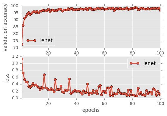

It is very interesting to see that the Simple Neural network starts off with a very high loss and low accuracy but eventually picks up the accuracy. Similarly, Simple NN2 also is in the middle of the Simple NN1 and the others indicating that the number of layers plays a very important role in how the network learns eventually and for lower epochs, a higher layer network should be chosen.
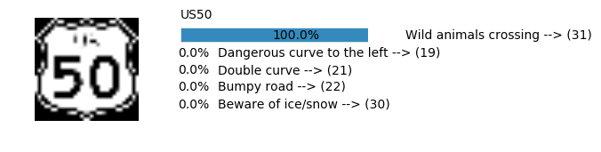
Step 3: Test a Model on New Images
I tested the model on about 5 images which look similar to the german traffic signs and the rest others which were randomly picked up from internet. Some of the images have never been seen before so it was interesting to how the different classifiers predicted the image. The one’s which looked similar to the german traffic signs were identified correctly by all networks
Load and Output the Images
total_images_from_internet = data.images_from_internet.shape[0]
i = 0
plt.figure(figsize=(12, 12))
total_rows = total_images_from_internet / 5 + 1
for img, filename in zip(data.images_from_internet, data.filenames_from_internet):
    plt.subplot(total_rows, 5, i+1)
    if img.shape[2] == 1:
        img = np.reshape(img, (32, 32))
    plt.imshow(img, cmap='gray')
    plt.axis('off')
    plt.title(filename.split(".")[0].split('/')[1])
    i += 1

plt.tight_layout()
plt.show()
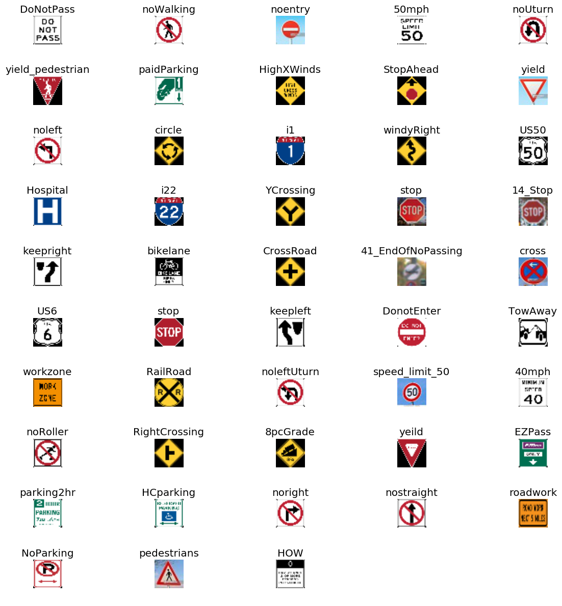
Discussion on Test Images
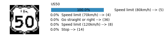
The test images I obtained were a mix of both german and US signs. The US signs had a different size than the german signs.
- German signs I got were of 32x32x3
- US Signs had different sizes and had to be resized to 32x32x3 for the models to work. Some images lost their aspect ratio because of this.
From the training and testing set we have seen that contrast of the image could affect the classification. Although I didn’t try histogram equalization, 2 of the DeepNet networks use 1x1 filters as the first layer which tend to make the contrast insignificant. The angle of the traffic sign shouldn’t be a big problem since our augmented data set already generates images based on random jittering between -10 and 10 degrees. Another thing to note is that all the images were cropped to include only the sign as the most significant object. However, that could pose a problem with images with backgrounds and I didn’t get a chance to test those. Some of the images are completely different from what the network has seen and hence it was evident that the none of the networks were able to classify them correctly.
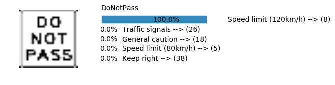
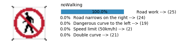
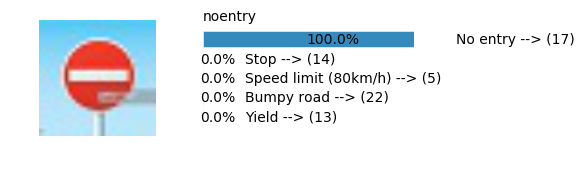
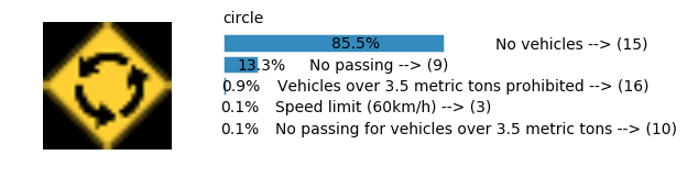
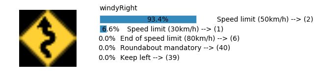
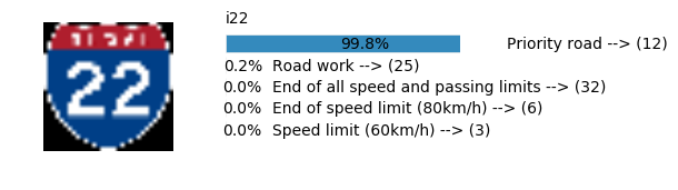
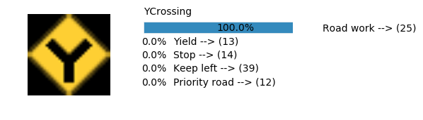
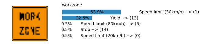
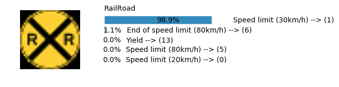
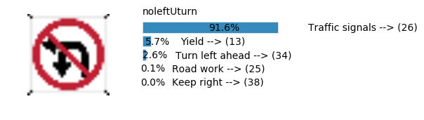
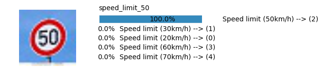
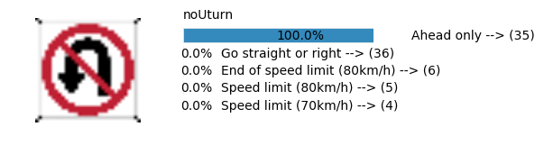
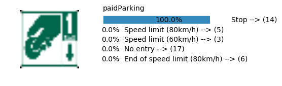
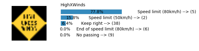
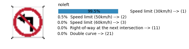
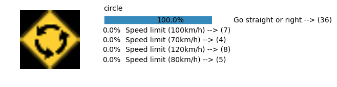
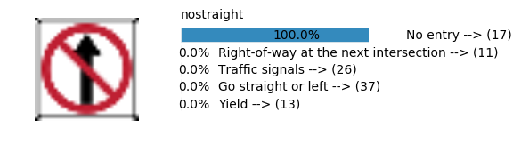
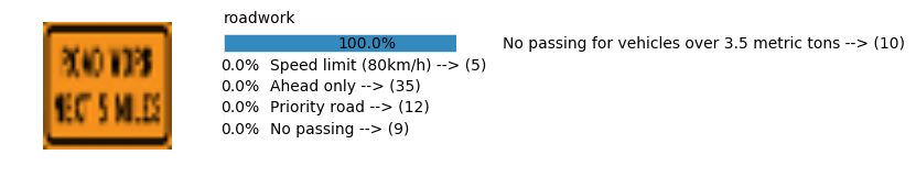
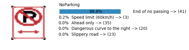
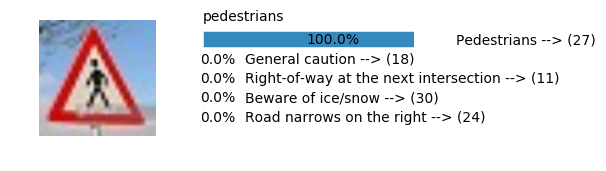
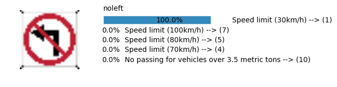
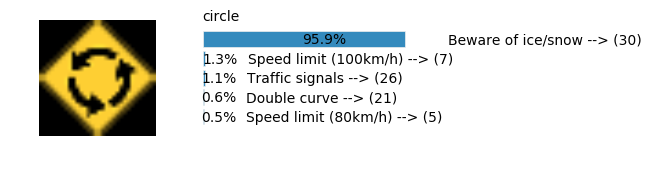
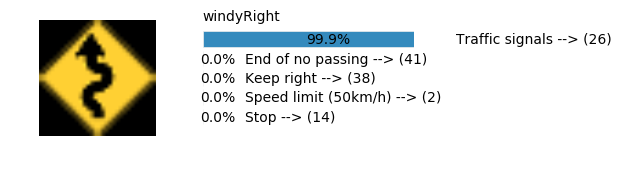
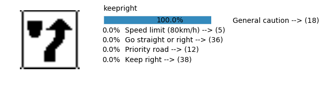
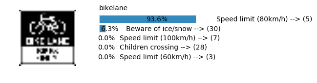
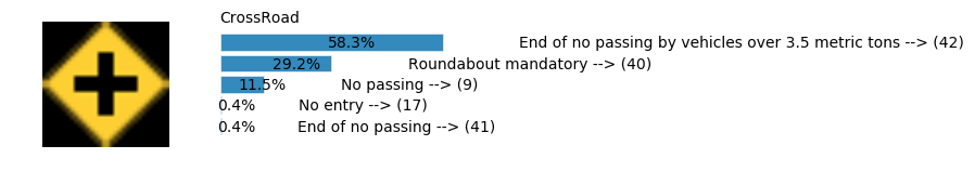
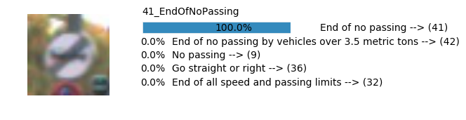
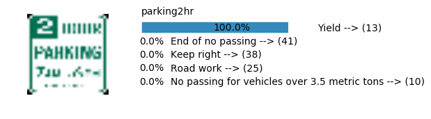
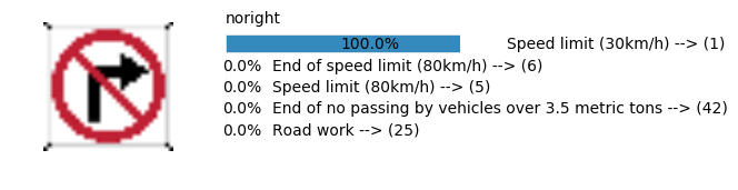
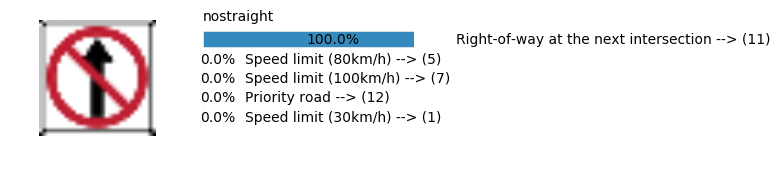
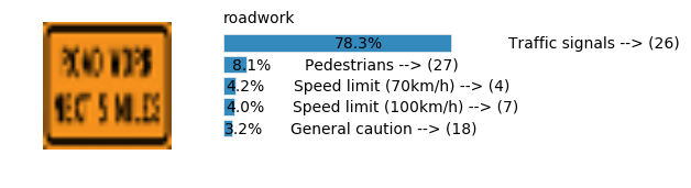
Prediction Function
import matplotlib.gridspec as gridspec
def predict(sess, tensor_ops, images, data, cfg, top_k=5):
print("Predicting from Random Images: Number of Images: %s" % images.shape[0])
print(images.shape)
cfg.IS_TRAINING = False
pred = tf.nn.softmax(tensor_ops.logits)
predictions = sess.run(pred, feed_dict={tensor_ops.x: images, tensor_ops.dropout_keep_prob: 1.0})
values, indices = tf.nn.top_k(predictions, top_k)
values, indices = values.eval(session=sess), indices.eval(session=sess)
print(values, indices)
filenames = data.filenames_from_internet
for i, img in enumerate(images):
plt.figure(figsize = (top_k, 1.5))
gs = gridspec.GridSpec(1, 2,width_ratios=[2,3])
plt.subplot(gs[0])
if img.shape[2] == 1:
img = np.reshape(img, (img.shape[0], img.shape[1]))
plt.imshow(img)
plt.axis('off')
plt.subplot(gs[1])
plt.barh(top_k + 1 - np.arange(top_k), values[i], align='center')
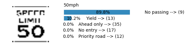
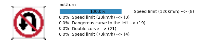
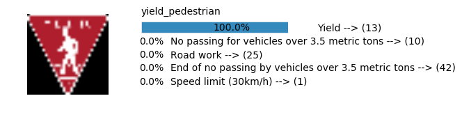
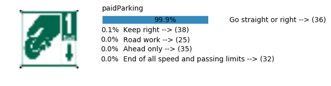
for i_label in range(top_k):
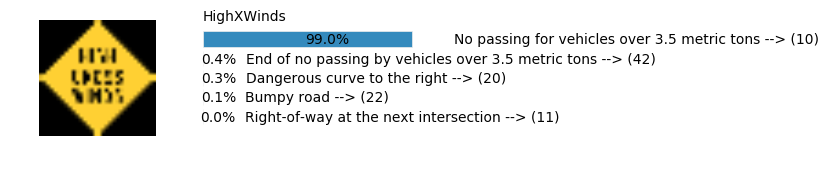
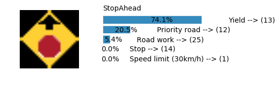
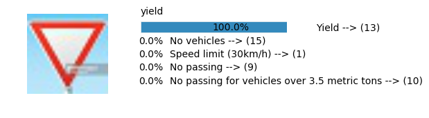
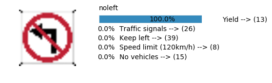
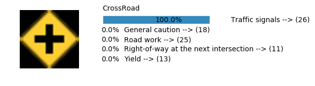
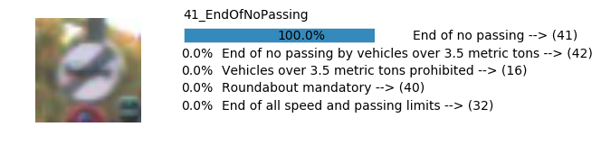
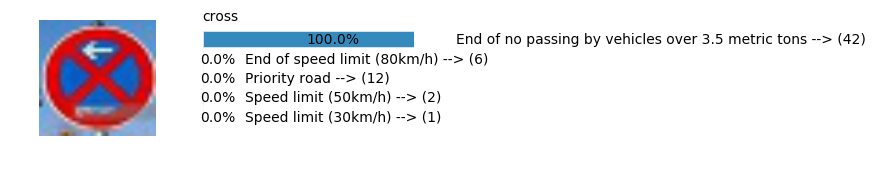
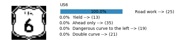
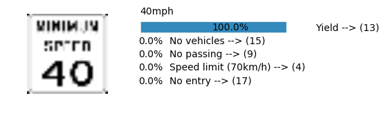
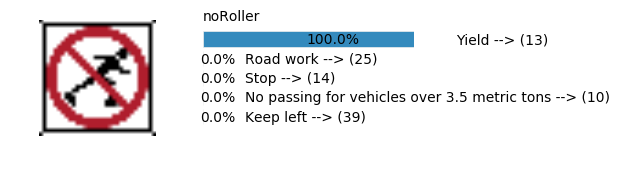
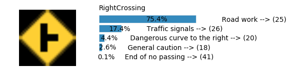
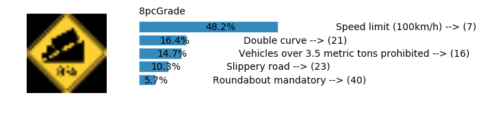
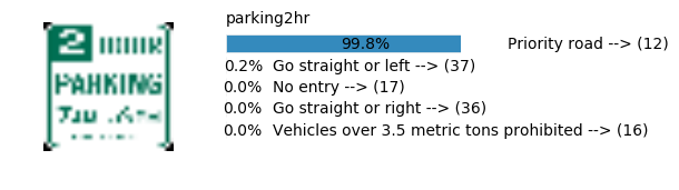
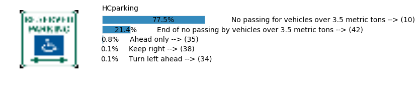
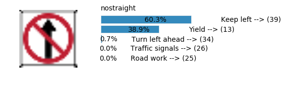
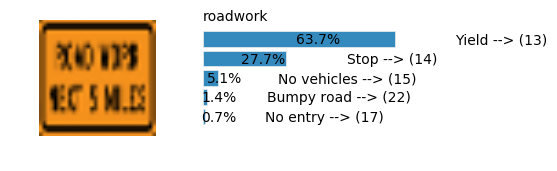
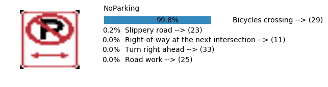
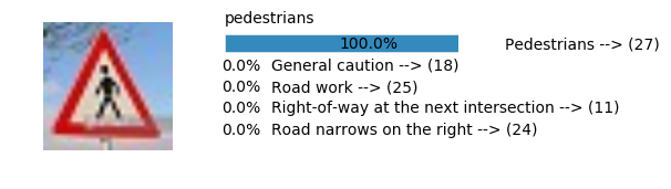
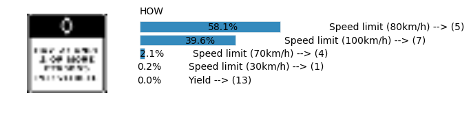
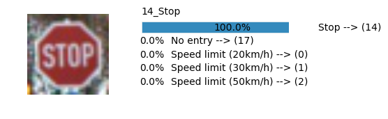
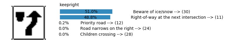
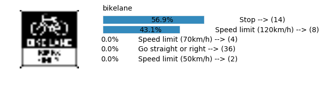
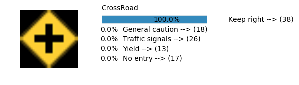
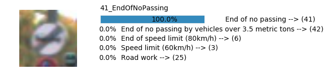
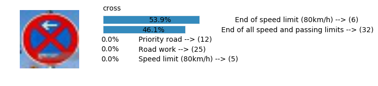
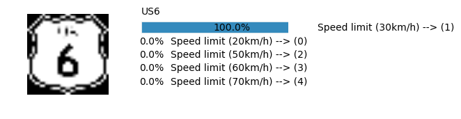
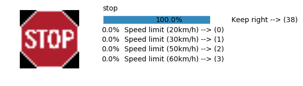
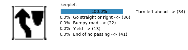
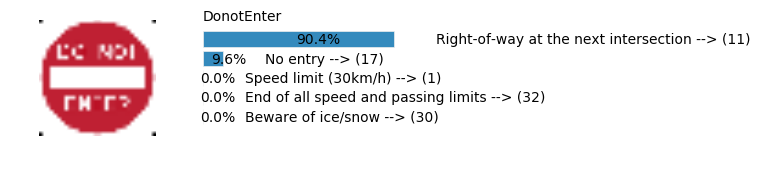
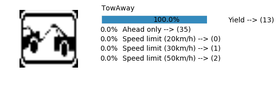
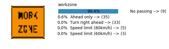
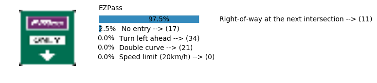
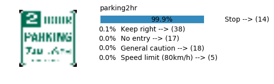
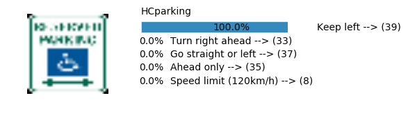
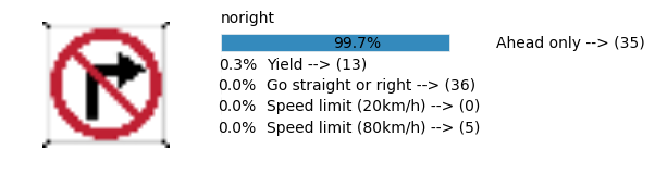
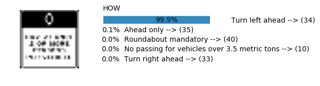
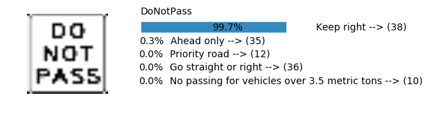
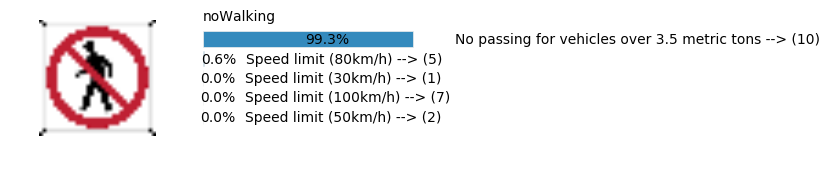
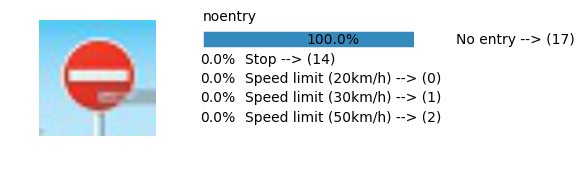
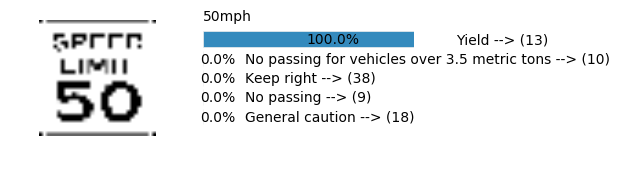
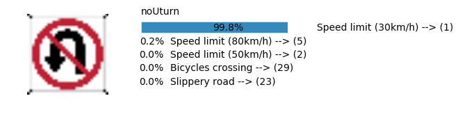
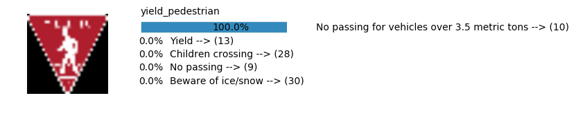
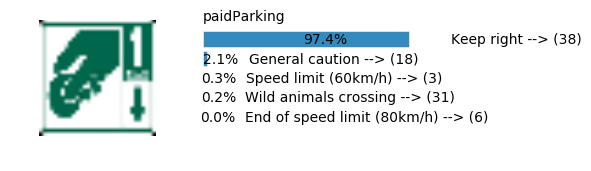
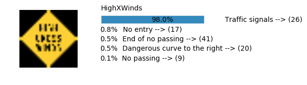
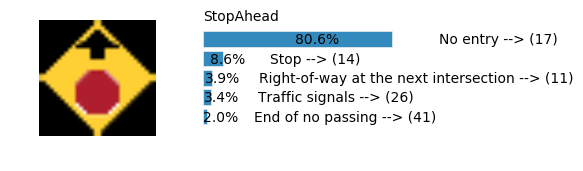
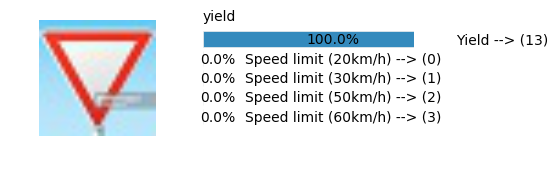
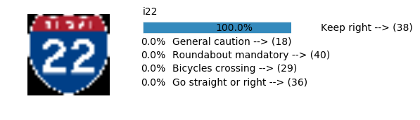
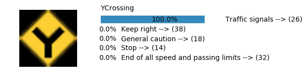
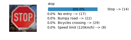
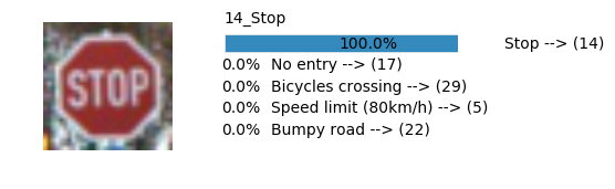
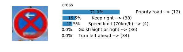
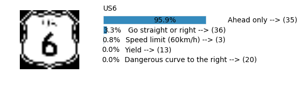
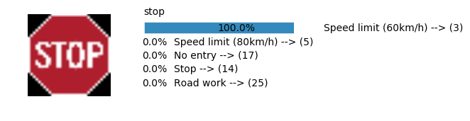
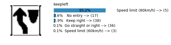
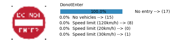
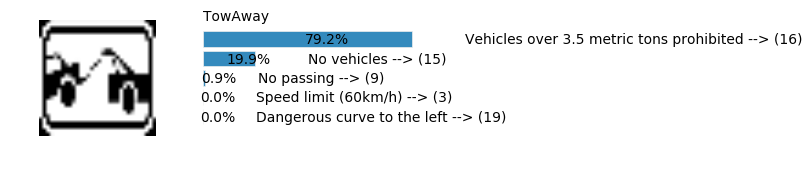
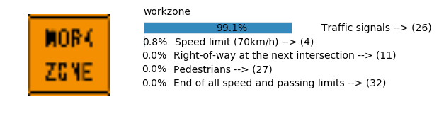
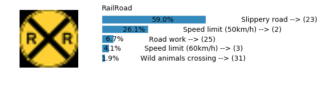
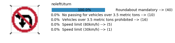
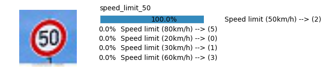
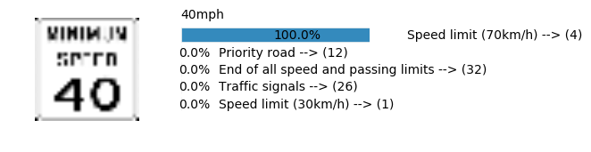
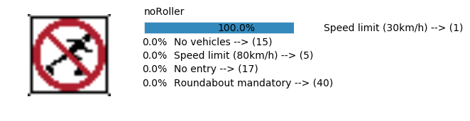
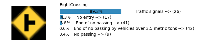
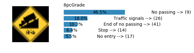
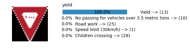
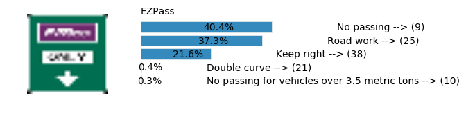
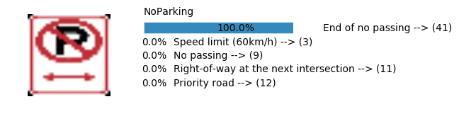
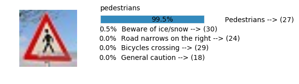
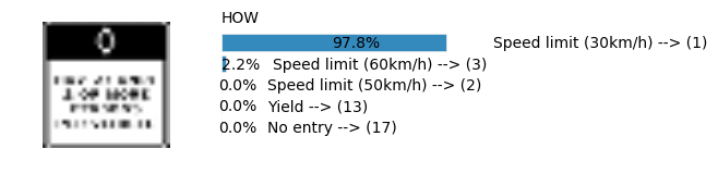
plt.text(values[i][i_label] + .2, top_k + 1-i_label-.25, data.get_signname(indices[i][i_label]) + " --> (" + str(indices[i][i_label]) + ")")
plt.text(values[i][i_label] / 2.0 - 0.01, top_k + 1-i_label-.25, "{:2.1f}%".format(values[i][i_label] * 100.0))
plt.axis('off');
plt.text(0,6.95, filenames[i].split(".")[0].split('/')[1]);
plt.show();
plt.show()
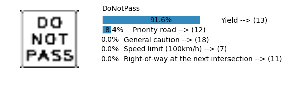
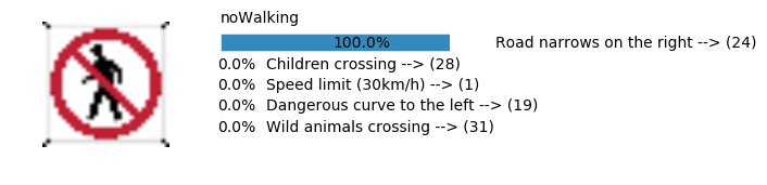
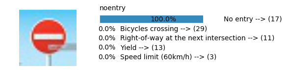
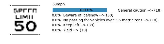
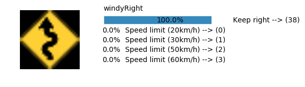
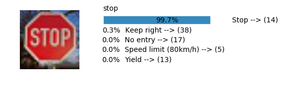
LeNet Prediction
sess, lenet_tensor_ops, data, cfg = train_and_test(preprocess=False, epochs=100, network="lenet", use_augmented_file=False, dropout_keep_prob=1.0)
predict(sess, lenet_tensor_ops, data.images_from_internet, data, cfg, top_k=5)
Predicting from Random Images: Number of Images: 48
(48, 32, 32, 3)
[[  9.99995947e-01   3.94990684e-06   5.32977396e-08   1.61552882e-10
    2.68203012e-11]
 [  9.99999881e-01   1.05881867e-07   4.22625650e-11   2.46448591e-11
    6.23271747e-12]
 [  1.00000000e+00   5.95051963e-21   2.31173243e-23   8.36679287e-24
    8.93535943e-25]
 [  8.97958815e-01   1.02041215e-01   4.67244092e-08   8.20396817e-09
    7.68765954e-11]
 [  1.00000000e+00   1.73554717e-08   1.74809756e-09   1.08864142e-11
    4.64379999e-13]
 [  1.00000000e+00   1.43294110e-09   1.37969480e-09   6.36412145e-10
    3.12190551e-10]
 [  9.98940051e-01   8.64406989e-04   1.95408444e-04   1.70211578e-07
    2.85503852e-08]
 [  9.89913464e-01   3.91400559e-03   3.42309871e-03   1.25362095e-03
    2.75771657e-04]
 [  7.40724623e-01   2.04770327e-01   5.43833748e-02   1.18617281e-04
    2.60742968e-06]
 [  1.00000000e+00   2.40315126e-31   6.91493956e-32   2.62442338e-33
    1.97547106e-34]
 [  1.00000000e+00   7.06153469e-11   1.36161317e-11   2.51960085e-12
    2.43252169e-13]
 [  8.54874015e-01   1.32682249e-01   9.31786094e-03   1.23101543e-03
    1.01866992e-03]
 [  1.00000000e+00   4.68930198e-16   4.44727814e-19   3.85083982e-19
    1.41763268e-21]
 [  9.33571339e-01   6.59451410e-02   4.11425688e-04   2.93423564e-05
    1.80204970e-05]
 [  1.00000000e+00   1.07756297e-10   2.38316108e-14   7.98440470e-18
    4.34123093e-24]
 [  1.00000000e+00   5.71778701e-11   2.59264262e-17   1.22059665e-17
    4.40439062e-21]
 [  9.98013496e-01   1.98217342e-03   4.23395250e-06   3.09266355e-08
    2.71086389e-08]
 [  9.99999166e-01   7.89297133e-07   1.39761958e-09   5.54279789e-10
    2.63311976e-11]
 [  9.97304082e-01   2.67575518e-03   1.21478288e-05   3.68276301e-06
    2.41076918e-06]
 [  1.00000000e+00   9.38881178e-12   2.93493832e-12   2.59336857e-14
    1.75077594e-14]
 [  8.74360383e-01   1.06773667e-01   1.44164125e-02   2.38470081e-03
    2.03138357e-03]
 [  9.88241613e-01   1.17136650e-02   2.12672476e-05   1.17064437e-05
    7.15414262e-06]
 [  9.99982834e-01   9.81424819e-06   5.98279439e-06   1.44285059e-06
    7.95869948e-09]
 [  9.99997020e-01   3.02176272e-06   7.49599839e-18   2.17371795e-18
    1.51705312e-19]
 [  9.99811351e-01   1.25955412e-04   4.22987105e-05   9.93310914e-06
    7.21907918e-06]
 [  1.00000000e+00   3.70743610e-23   2.38045168e-23   8.32114859e-24
    8.11885518e-29]
 [  6.57242298e-01   1.47824451e-01   1.00293927e-01   9.21592414e-02
    1.43983157e-03]
 [  5.40124178e-01   2.86305726e-01   1.24741413e-01   2.01201309e-02
    1.55694885e-02]
 [  1.00000000e+00   9.06478191e-12   1.22549627e-12   1.06119172e-12
    7.47644473e-14]
 [  1.00000000e+00   1.99300008e-13   2.31418761e-21   1.52519642e-22
    1.99953883e-23]
 [  6.39385521e-01   3.25981498e-01   4.84234700e-03   4.68484918e-03
    4.53225942e-03]
 [  9.88660336e-01   1.12433825e-02   8.54731625e-05   3.42083081e-06
    3.02991975e-06]
 [  9.16259706e-01   5.67104667e-02   2.62487624e-02   5.52572077e-04
    2.25997050e-04]
 [  1.00000000e+00   1.68816549e-32   0.00000000e+00   0.00000000e+00
    0.00000000e+00]
 [  1.00000000e+00   1.64732353e-10   1.05275596e-21   7.84693637e-23
    3.70017385e-23]
 [  9.99882936e-01   1.17102783e-04   3.37436052e-13   2.20175932e-14
    2.80006159e-15]
 [  7.54247904e-01   1.73664212e-01   4.43104170e-02   2.57580448e-02
    7.24208076e-04]
 [  4.81678247e-01   1.63846433e-01   1.46945313e-01   1.03002325e-01
    5.73947132e-02]
 [  1.00000000e+00   8.14832478e-23   1.04826142e-25   1.76975459e-26
    3.62220969e-27]
 [  1.00000000e+00   2.73842782e-10   1.30853224e-14   4.34295471e-16
    2.91356464e-16]
 [  9.97853577e-01   1.88243075e-03   2.51716352e-04   1.08583990e-05
    5.25192775e-07]
 [  7.74930000e-01   2.13943705e-01   8.39991216e-03   1.10920775e-03
    8.45671922e-04]
 [  8.16304684e-01   7.37141743e-02   6.97023124e-02   3.88607979e-02
    1.31491711e-03]
 [  6.03187978e-01   3.89151156e-01   7.41862366e-03   7.71263221e-05
    6.68781504e-05]
 [  6.36888742e-01   2.76924908e-01   5.07784784e-02   1.43415490e-02
    6.96288375e-03]
 [  9.98354971e-01   1.58469507e-03   5.39483954e-05   5.30342277e-06
    6.75886042e-07]
 [  9.99992132e-01   7.92273840e-06   1.57962809e-11   6.57078038e-12
    2.36470474e-14]
 [  5.81149697e-01   3.95661622e-01   2.07017660e-02   2.29231943e-03
    9.82917045e-05]] [[ 8 26 18  5 38]
 [25 24 19  2 21]
 [17 14  5 22 13]
 [ 9 13 35 17 12]
 [ 8  0 19 21  4]
 [13 10 25 42  1]
 [36 38 25 35 32]
 [10 42 20 22 11]
 [13 12 25 14  1]
 [13 15  1  9 10]
 [13 26 39  8 15]
 [15  9 16  3 10]
 [35 36 24 33 40]
 [ 2  1  6 40 39]
 [ 4  1  0 18 24]
 [13 34 38 17 15]
 [12 25 32  6  3]
 [25 13 14 39 12]
 [14 25 32  1 39]
 [14 13 25 32 12]
 [11 40 21 19 34]
 [40 12 41 17 34]
 [26 18 25 11 13]
 [41 42 16 40 32]
 [42  6 12  2  1]
 [25 13 35 19 21]
 [14 13  6  1 39]
 [13 17 15  9 19]
 [17  4 22 13 15]
 [13  4 39  1 14]
 [ 1 13  5 14  0]
 [ 1  6 13  5  0]
 [26 13 34 25 38]
 [ 2  1  0  3  4]
 [13 15  9  4 17]
 [13 25 14 10 39]
 [25 26 20 18 41]
 [ 7 21 16 23 40]
 [13 15 26  4  9]
 [17 13 29 22 14]
 [12 37 17 36 16]
 [10 42 35 38 34]
 [24 22 39 26  2]
 [39 13 34 26 25]
 [13 14 15 22 17]
 [29 23 11 33 25]
 [27 18 25 11 24]
 [ 5  7  4  1 13]]


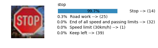
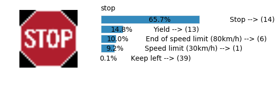
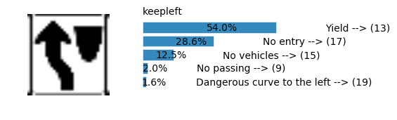
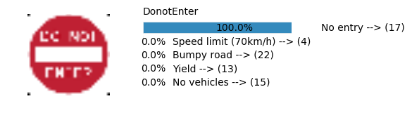
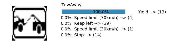


Accuracy
- Validation Accuracy: ~98%
- Testing Accuracy: 91.4%
- Real World Accuracy: 11 out of 48 images (~23%)
The reason the network didn’t perform well on these images is because signs of these categories were not included in the training set.
Simple NN 1 Prediction
sess, lenet_tensor_ops, data, cfg = train_and_test(preprocess=False, epochs=100, network="simple_nn1", use_augmented_file=False)
predict(sess, lenet_tensor_ops, data.images_from_internet, data, cfg, top_k=5)
Predicting from Random Images: Number of Images: 48
(48, 32, 32, 3)
[[  9.15771902e-01   8.37622657e-02   4.56795562e-04   9.01217754e-06
    3.86747212e-09]
 [  1.00000000e+00   1.91837567e-13   2.04673179e-14   4.99678712e-15
    2.60089540e-16]
 [  1.00000000e+00   1.11894077e-12   4.94399492e-25   2.71130723e-26
    2.10672948e-29]
 [  9.99999881e-01   6.72660292e-08   5.20649604e-13   6.46207788e-16
    4.50688596e-17]
 [  1.00000000e+00   2.58339331e-16   5.62767823e-27   1.68406528e-28
    3.87280837e-32]
 [  1.00000000e+00   4.54287674e-09   3.78711104e-16   4.39830494e-17
    3.09875192e-17]
 [  9.99995351e-01   4.69236420e-06   4.53218158e-14   2.44820304e-15
    7.80532899e-19]
 [  7.77718306e-01   1.58321619e-01   6.39396608e-02   2.01808925e-05
    2.76664963e-07]
 [  1.00000000e+00   6.85156690e-21   1.89185324e-32   0.00000000e+00
    0.00000000e+00]
 [  1.00000000e+00   0.00000000e+00   0.00000000e+00   0.00000000e+00
    0.00000000e+00]
 [  9.95290756e-01   4.70909802e-03   1.69977085e-07   1.64985525e-10
    5.49032564e-12]
 [  9.99988914e-01   1.11325699e-05   2.08339818e-10   2.92439684e-11
    6.89107582e-12]
 [  1.00000000e+00   4.92674261e-13   1.76715576e-13   3.00438616e-18
    2.49733894e-23]
 [  1.00000000e+00   0.00000000e+00   0.00000000e+00   0.00000000e+00
    0.00000000e+00]
 [  1.00000000e+00   1.66658315e-17   5.44047806e-22   6.00085936e-26
    1.22229105e-27]
 [  1.00000000e+00   5.38262475e-26   1.11671061e-27   1.09639879e-27
    8.70631172e-28]
 [  1.00000000e+00   8.07052198e-16   3.74702357e-21   8.46286520e-32
    4.37801447e-33]
 [  1.00000000e+00   3.58817900e-08   2.99283293e-18   2.48958507e-32
    0.00000000e+00]
 [  9.96807098e-01   3.19287018e-03   3.03202342e-12   2.80411074e-19
    6.68927197e-20]
 [  1.00000000e+00   3.62304799e-37   0.00000000e+00   0.00000000e+00
    0.00000000e+00]
 [  5.10020673e-01   4.88458067e-01   1.52086758e-03   4.58194307e-07
    4.63412558e-10]
 [  5.68647861e-01   4.31352109e-01   5.33712319e-09   2.95031020e-15
    4.06484031e-17]
 [  1.00000000e+00   8.56242899e-09   1.12121989e-09   9.54205411e-26
    7.84996181e-30]
 [  1.00000000e+00   1.89984431e-10   6.42262285e-12   3.57055791e-12
    2.56067872e-13]
 [  5.39052844e-01   4.60946202e-01   9.96867357e-07   7.10607449e-15
    2.24456214e-16]
 [  1.00000000e+00   2.98818599e-28   0.00000000e+00   0.00000000e+00
    0.00000000e+00]
 [  1.00000000e+00   0.00000000e+00   0.00000000e+00   0.00000000e+00
    0.00000000e+00]
 [  9.99829769e-01   1.68156548e-04   2.05542779e-06   4.46506859e-10
    1.03759293e-10]
 [  9.03711379e-01   9.62880105e-02   5.61909417e-07   5.99698182e-23
    2.39843313e-26]
 [  1.00000000e+00   4.40844305e-28   0.00000000e+00   0.00000000e+00
    0.00000000e+00]
 [  9.93866622e-01   6.13254216e-03   7.18106776e-07   8.50459472e-08
    3.54055238e-08]
 [  1.00000000e+00   3.67998460e-25   0.00000000e+00   0.00000000e+00
    0.00000000e+00]
 [  1.00000000e+00   9.84314366e-12   1.37343033e-20   3.01050686e-29
    1.22793822e-32]
 [  1.00000000e+00   7.02101311e-12   1.03570564e-24   6.62138636e-37
    0.00000000e+00]
 [  9.99999881e-01   9.48429388e-08   2.45517651e-08   2.44200162e-08
    2.41986076e-09]
 [  9.98748660e-01   8.06631637e-04   4.42888821e-04   1.27591511e-06
    5.10105451e-07]
 [  9.99997139e-01   2.82294991e-06   1.71783032e-08   2.37364052e-11
    4.48804709e-12]
 [  9.27891910e-01   4.04008776e-02   3.01908311e-02   1.51603529e-03
    3.62978682e-07]
 [  1.00000000e+00   6.88834920e-17   5.65874309e-19   5.39298185e-19
    6.39930883e-22]
 [  9.75441337e-01   2.45587025e-02   4.05929370e-12   7.31974192e-18
    1.13665225e-18]
 [  9.99432504e-01   5.67517709e-04   3.06344170e-13   6.29328133e-14
    5.71699738e-14]
 [  9.99992728e-01   7.28142049e-06   1.64795705e-12   5.51790167e-13
    2.29119649e-17]
 [  9.97247636e-01   2.75229779e-03   7.32435339e-08   1.04493169e-14
    8.28288278e-15]
 [  9.99997258e-01   2.29327452e-06   4.99525015e-07   5.86246856e-08
    5.63908529e-08]
 [  9.99999881e-01   1.48996463e-07   1.37816212e-08   1.29777122e-08
    1.88655669e-09]
 [  9.98105049e-01   1.86118507e-03   3.37196798e-05   5.86585713e-08
    1.35852964e-08]
 [  1.00000000e+00   2.54107237e-16   7.75953516e-17   1.39033970e-22
    2.29477037e-27]
 [  9.99205530e-01   7.52609165e-04   4.07984553e-05   1.06246932e-06
    3.16055741e-14]] [[13 12 18  7 11]
 [24 28  1 19 31]
 [17 29 11 13  3]
 [18 30 10 39 13]
 [35 36  6  5  4]
 [13 35 39 33  9]
 [14  5  3 17  6]
 [ 5  2 38  6  9]
 [12 13 38  0  1]
 [13  0  1  2  3]
 [ 1  2  3 11 21]
 [36  7  4  8  5]
 [35  5 13  3 36]
 [38  0  1  2  3]
 [ 5  4 36  8 14]
 [34 36 29 12 11]
 [33  9 26 12 39]
 [ 7 40  1  2  0]
 [14 38 17  5 13]
 [14 17  0  1  2]
 [30 11 12 24 28]
 [14  8  4 36  2]
 [38 18 26 13 17]
 [41 42  6  3 25]
 [ 6 32 12 25  5]
 [ 1  0  2  3  4]
 [38  0  1  2  3]
 [34 36 22 13 41]
 [11 17  1 32 30]
 [13 35  0  1  2]
 [ 9 35 33  5  3]
 [ 4  1  0  2  3]
 [35 13 39 24  1]
 [ 2  5  1  3  0]
 [32 35  3  6 11]
 [33  5  1  4  6]
 [38 17  4  1 20]
 [ 3  7  5 16 10]
 [13 12 14 35 23]
 [11 17 34 21  0]
 [14 38 17 18  5]
 [39 33 37 35  8]
 [35 13 36  0  5]
 [17 11 26 37 13]
 [10  5 35 12  9]
 [41  3 35 20 23]
 [27 18 11 30 24]
 [34 35 40 10 33]]


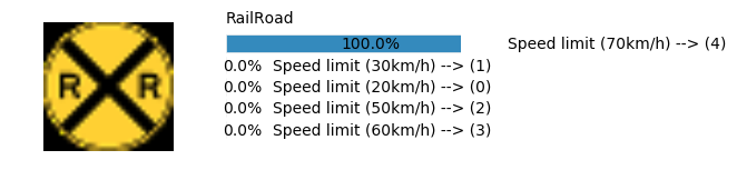
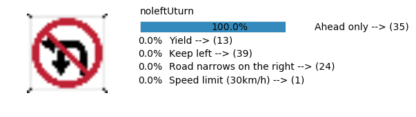

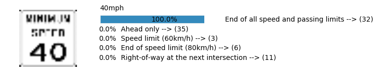

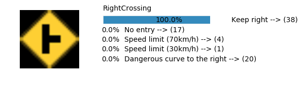


Accuracy
- Validation Accuracy: ~94%
- Testing Accuracy: 84.7%
- Real World Accuracy: 11 out of 48 images (~23%)
The reason the network didn’t perform well on these images is because signs of these categories were not included in the training set.
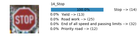
Simple NN 2 Prediction
sess, lenet_tensor_ops, data, cfg = train_and_test(preprocess=False, epochs=100, network="simple_nn2", use_augmented_file=False)
predict(sess, lenet_tensor_ops, data.images_from_internet, data, cfg, top_k=5)
Predicting from Random Images: Number of Images: 48
(48, 32, 32, 3)
[[  9.97232974e-01   2.71830475e-03   4.35913971e-05   5.02739476e-06
    1.49079000e-07]
 [  9.93392527e-01   6.28122734e-03   1.65314617e-04   1.60904616e-04
    3.14810785e-15]
 [  1.00000000e+00   1.26103182e-29   0.00000000e+00   0.00000000e+00
    0.00000000e+00]
 [  1.00000000e+00   2.80141840e-20   9.83983280e-21   1.20507094e-23
    1.77913649e-26]
 [  9.97579634e-01   2.31008325e-03   1.09923960e-04   2.79316168e-07
    2.67776812e-07]
 [  1.00000000e+00   9.83909412e-11   2.09444160e-14   5.56303881e-15
    7.08395147e-16]
 [  9.74317968e-01   2.09395215e-02   2.84518045e-03   1.71985349e-03
    1.70302039e-04]
 [  9.80245173e-01   7.62314862e-03   5.01776347e-03   4.78735287e-03
    7.38579081e-04]
 [  8.06260407e-01   8.61391649e-02   3.94311398e-02   3.41650546e-02
    1.96643528e-02]
 [  1.00000000e+00   0.00000000e+00   0.00000000e+00   0.00000000e+00
    0.00000000e+00]
 [  9.99986768e-01   1.32724754e-05   2.76073088e-11   7.55116431e-19
    3.16024637e-19]
 [  9.59310591e-01   1.31634651e-02   1.08417552e-02   5.90662472e-03
    5.47168963e-03]
 [  1.00000000e+00   1.51107360e-12   4.70413073e-26   4.10230541e-29
    6.93285503e-30]
 [  9.98742521e-01   3.40826024e-04   2.64952163e-04   7.08049629e-05
    7.05326238e-05]
 [  1.00000000e+00   5.54329453e-08   4.29826147e-10   2.40088054e-11
    1.34210733e-11]
 [  9.97585654e-01   2.41429755e-03   4.17752277e-09   1.20138968e-18
    6.29537825e-20]
 [  9.99997973e-01   2.07124162e-06   4.87651235e-08   7.92795873e-09
    4.26128244e-10]
 [  9.99752104e-01   7.84839212e-05   3.77066281e-05   3.10515206e-05
    1.20149016e-05]
 [  1.00000000e+00   2.94336569e-11   1.36529924e-17   1.93134534e-18
    7.14772648e-20]
 [  1.00000000e+00   1.75886597e-25   1.16309923e-31   2.14451018e-33
    1.66331771e-33]
 [  9.99996424e-01   3.50982305e-06   1.23837305e-08   1.60899807e-10
    4.44709373e-11]
 [  9.36192811e-01   6.32947981e-02   3.29692441e-04   1.47813713e-04
    3.09071802e-05]
 [  5.82951725e-01   2.91624188e-01   1.15124926e-01   4.10299515e-03
    3.54081881e-03]
 [  1.00000000e+00   7.16128707e-21   4.84268406e-22   8.46725904e-24
    5.63578304e-25]
 [  7.09769845e-01   1.65077657e-01   1.24724150e-01   4.11071873e-04
    1.73032222e-05]
 [  9.58758891e-01   3.34299356e-02   7.61258835e-03   1.11843699e-04
    6.13955053e-05]
 [  1.00000000e+00   1.22997185e-11   4.39587830e-22   3.19108814e-23
    9.53037189e-27]
 [  9.32123661e-01   3.59844230e-02   2.92879045e-02   1.37214595e-03
    9.85280029e-04]
 [  1.00000000e+00   5.69172774e-37   8.96709048e-38   0.00000000e+00
    0.00000000e+00]
 [  7.92147994e-01   1.98691368e-01   9.01786890e-03   1.42683333e-04
    1.60054263e-08]
 [  9.90897954e-01   8.09980743e-03   3.36969504e-04   2.99725914e-04
    1.14055118e-04]
 [  5.89608312e-01   2.61126727e-01   6.69967905e-02   4.14078012e-02
    1.93488430e-02]
 [  9.99981642e-01   1.83786142e-05   1.40792868e-12   6.03466929e-14
    2.79557062e-20]
 [  1.00000000e+00   2.12253485e-19   0.00000000e+00   0.00000000e+00
    0.00000000e+00]
 [  1.00000000e+00   6.90564272e-11   5.06542464e-12   2.77448691e-15
    3.54545327e-17]
 [  1.00000000e+00   2.49906467e-11   2.20979485e-12   1.01837873e-14
    1.79401631e-16]
 [  8.93274844e-01   4.26391512e-02   3.75375077e-02   5.51539892e-03
    4.37198253e-03]
 [  4.65010762e-01   1.80185720e-01   1.03130445e-01   6.36947453e-02
    5.49868569e-02]
 [  1.00000000e+00   3.17991571e-11   1.67637735e-24   1.98464808e-27
    5.06660120e-28]
 [  4.04035866e-01   3.73209834e-01   2.15642437e-01   3.69974854e-03
    2.70580407e-03]
 [  9.99999523e-01   2.53607624e-07   1.29951019e-07   7.51913802e-08
    1.02625596e-10]
 [  9.92475450e-01   7.52205867e-03   1.66642883e-06   8.62881279e-07
    1.41770435e-08]
 [  9.99986410e-01   1.35847295e-05   4.27943370e-08   2.50462693e-12
    1.31014427e-12]
 [  9.99823034e-01   1.72405315e-04   3.99679766e-06   2.47897503e-07
    2.32679241e-07]
 [  7.83443689e-01   8.08533728e-02   4.18982208e-02   3.97728346e-02
    3.19895670e-02]
 [  9.99998569e-01   8.63282366e-07   3.57163799e-07   1.53000173e-07
    1.14723145e-13]
 [  9.95355368e-01   4.64467611e-03   1.57733791e-11   2.81908221e-12
    2.38228474e-14]
 [  9.78138208e-01   2.18529645e-02   6.95642348e-06   8.91755519e-07
    6.20688411e-07]] [[38 35 12 36 10]
 [10  5  1  7  2]
 [17 14  0  1  2]
 [13 10 38  9 18]
 [ 1  5  2 29 23]
 [10 13 28  9 30]
 [38 18  3 31  6]
 [26 17 41 20  9]
 [17 14 11 26 41]
 [13  0  1  2  3]
 [ 1  7  5  4 10]
 [30  7 26 21  5]
 [35 36 34 12 21]
 [26 41 38  2 14]
 [31 19 21 22 30]
 [23 30  3 33 17]
 [38 18 40 29 36]
 [26 38 18 14 32]
 [14 17 22 29  8]
 [14 17 29  5 22]
 [18  5 36 12 38]
 [ 5 30  7 28  3]
 [42 40  9 17 41]
 [41 42  9 36 32]
 [12 38  4 36 34]
 [35 36  3 13 20]
 [ 3  5 17 14 25]
 [ 5 17 38 36  3]
 [17 15  8  0  1]
 [16 15  9  3 19]
 [26  4 11 27 32]
 [23  2 25  3 31]
 [40 10 16  5  1]
 [ 2  5  0  1  3]
 [ 4 12 32 26  1]
 [ 1 15  5 17 40]
 [26 17 41 42  9]
 [ 9 26 41 14 17]
 [13 10 25  1 28]
 [ 9 25 38 21 10]
 [13 41 38 25 10]
 [34 38 18 35  4]
 [ 1  6  5 42 25]
 [11  5  7 12  1]
 [26 27  4  7 18]
 [41  3  9 11 12]
 [27 30 24 29 18]
 [ 1  3  2 13 17]]


Accuracy
- Validation Accuracy: ~98.7%
- Testing Accuracy: 92.4%
- Real World Accuracy: 11 out of 48 images (~23%)
The reason the network didn’t perform well on these images is because signs of these categories were not included in the training set.
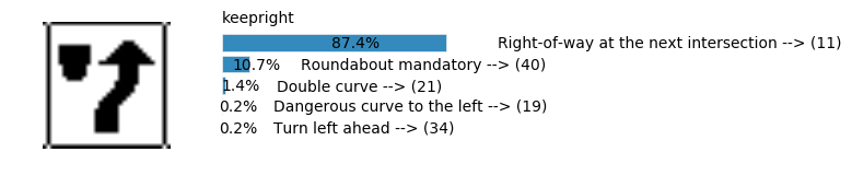
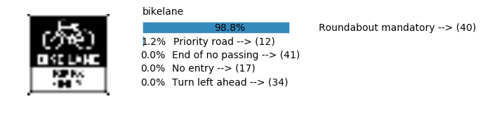
DeepNet Merge Layers Prediction
sess, lenet_tensor_ops, data, cfg = train_and_test(preprocess=False, dropout_keep_prob = 0.5, epochs=100, network="deepnetmergelayers", use_augmented_file=False)
predict(sess, lenet_tensor_ops, data.images_from_internet, data, cfg, top_k=5)
Predicting from Random Images: Number of Images: 48
(48, 32, 32, 3)
[[  9.97562647e-01   1.90260913e-03   4.71238338e-04   4.17677365e-05
    1.27778867e-05]
 [  3.88801843e-01   3.48304749e-01   2.42090821e-01   7.69898528e-03
    3.89499892e-03]
 [  9.99997377e-01   2.09160589e-06   5.11241240e-07   3.86604984e-11
    3.31054385e-11]
 [  9.99517798e-01   4.81176568e-04   9.11421751e-07   1.30105505e-07
    3.24600613e-08]
 [  9.95575070e-01   2.36847368e-03   1.29205734e-03   5.55386418e-04
    7.94104126e-05]
 [  9.99989986e-01   9.81671474e-06   2.21197965e-07   4.78848818e-08
    1.37493474e-08]
 [  7.77554095e-01   7.42456540e-02   6.81248233e-02   5.97214177e-02
    1.85023677e-02]
 [  4.76081520e-01   3.32262754e-01   7.80436695e-02   5.55680208e-02
    3.90291475e-02]
 [  9.81861472e-01   1.41060222e-02   3.69121297e-03   1.09894158e-04
    6.92193498e-05]
 [  1.00000000e+00   1.98422700e-09   9.11771381e-10   2.47231575e-11
    1.75938517e-11]
 [  9.93728638e-01   1.22157275e-03   1.08479615e-03   1.04239432e-03
    1.01205905e-03]
 [  3.98666829e-01   1.16061904e-01   1.11650214e-01   9.65233892e-02
    8.28552321e-02]
 [  5.13597250e-01   2.23120824e-01   1.59660414e-01   9.55395550e-02
    4.55814740e-03]
 [  3.96058917e-01   2.10823536e-01   7.30365217e-02   3.44145745e-02
    3.16597000e-02]
 [  9.99925494e-01   6.90002780e-05   1.91423760e-06   1.84812325e-06
    8.66665630e-07]
 [  5.82450986e-01   4.17548716e-01   1.66931798e-07   8.97878820e-08
    2.21953877e-09]
 [  8.31328809e-01   9.71229151e-02   5.29605746e-02   1.09427208e-02
    2.95406696e-03]
 [  8.06191742e-01   1.06564112e-01   4.00067084e-02   7.81072304e-03
    4.12366400e-03]
 [  9.98511612e-01   1.44653034e-03   2.25641088e-05   1.69182676e-05
    1.54216673e-06]
 [  1.00000000e+00   2.86370405e-16   5.93409710e-17   6.02795629e-18
    6.63307344e-20]
 [  9.98785913e-01   9.05659399e-04   2.65728362e-04   2.71096978e-05
    6.31073226e-06]
 [  4.45657700e-01   2.25300401e-01   1.66521534e-01   5.20843789e-02
    2.08428875e-02]
 [  7.63750255e-01   6.42739311e-02   3.07866950e-02   2.29985639e-02
    2.04569027e-02]
 [  9.99999642e-01   1.90403284e-07   1.02063773e-07   1.53580046e-08
    1.17457521e-09]
 [  8.51134241e-01   1.35426924e-01   3.73149640e-03   3.05346772e-03
    1.63827906e-03]
 [  4.61883396e-01   3.37018639e-01   1.59364656e-01   2.41845306e-02
    7.74752721e-03]
 [  7.84145236e-01   1.27853245e-01   4.94942255e-02   2.47998331e-02
    1.04228090e-02]
 [  8.66155624e-01   1.25383839e-01   4.53886902e-03   1.51721446e-03
    1.19717291e-03]
 [  9.82465088e-01   1.73125975e-02   1.02621671e-04   4.13756097e-05
    3.52259412e-05]
 [  9.82005119e-01   9.46321525e-03   5.73994406e-03   2.37746094e-03
    3.76010081e-04]
 [  2.83116281e-01   1.99584603e-01   1.88389540e-01   1.15102693e-01
    7.39458725e-02]
 [  5.52131057e-01   1.28297746e-01   4.05201539e-02   2.94880234e-02
    2.36666556e-02]
 [  5.57871103e-01   2.35774234e-01   1.32786140e-01   2.85325032e-02
    8.57422408e-03]
 [  1.00000000e+00   1.30109167e-13   4.47856372e-14   2.51448888e-15
    1.11661939e-15]
 [  9.99756157e-01   7.92738792e-05   7.16862487e-05   4.91493302e-05
    2.72516700e-05]
 [  9.99791801e-01   1.15491996e-04   6.60617807e-05   2.38468529e-05
    9.58928922e-07]
 [  4.56001937e-01   1.03275642e-01   8.54945108e-02   7.96180367e-02
    5.78075163e-02]
 [  5.06141305e-01   8.21096599e-02   4.75059189e-02   3.87558937e-02
    3.41528133e-02]
 [  9.99999285e-01   6.60221929e-07   4.42001884e-08   2.99274312e-08
    2.11082902e-08]
 [  5.92440486e-01   3.61626983e-01   3.90484333e-02   3.95678449e-03
    5.33011334e-04]
 [  9.99997616e-01   2.37518498e-06   3.78245417e-08   3.11809134e-09
    1.95249505e-09]
 [  8.70135188e-01   1.23016588e-01   4.15246701e-03   1.13003235e-03
    5.60075452e-04]
 [  9.41634119e-01   4.59520780e-02   9.00954194e-03   2.41636136e-03
    3.12482007e-04]
 [  7.99433589e-01   1.72333732e-01   1.97483171e-02   3.42057133e-03
    1.36006449e-03]
 [  6.86615407e-01   1.31146803e-01   5.76779917e-02   3.85195911e-02
    1.39067862e-02]
 [  7.46641338e-01   1.41465858e-01   9.24468413e-02   1.64253488e-02
    1.05720921e-03]
 [  9.85954702e-01   1.40432483e-02   1.93403162e-06   9.02174904e-08
    7.22188034e-08]
 [  9.06346083e-01   6.95231482e-02   1.24595724e-02   6.05744310e-03
    1.53907645e-03]] [[40  9 38 23 41]
 [ 1 29 21 42 40]
 [17  9 10 14 29]
 [13 40  9 12 23]
 [20 25 32 41 42]
 [13  1  9 33 14]
 [ 1  6 38  2 41]
 [10  9 14 17 12]
 [12 10  9 17 25]
 [13 15 12 22  1]
 [ 2 25 41 19 15]
 [ 7 14 15 12 13]
 [35 25  1 39 22]
 [12  4 25  2 19]
 [35  1 36 39 25]
 [35 13 34 33  1]
 [11 40  1 23 39]
 [13 38 12 11 32]
 [14 17 15  1  9]
 [14 17 15  9  1]
 [39 40 38 37 33]
 [11 38  2 35 39]
 [11 40 35  7 39]
 [41 42  9 40 16]
 [ 1 29 42 12 20]
 [19  4 35  1 39]
 [13 25  6 14 17]
 [13 38 12 39 33]
 [13 15 11 35  1]
 [12 40 10 13 35]
 [13 12 29 15  9]
 [ 6 25 13  5 42]
 [ 6 15  1 40  0]
 [ 2 37  1  4  7]
 [13  1 40 17 15]
 [ 1 12 10 40 25]
 [42 12 40 20 13]
 [13  7  1  8 21]
 [13  1 11  9 12]
 [38 12 25 13 23]
 [25 22 12 10 36]
 [37 39 40 12 30]
 [ 6 17 25 38 42]
 [15 18  1 14 40]
 [13  1 14 25 38]
 [ 6 41 23 42 11]
 [27 18 11 24  1]
 [ 3  6 38 39 23]]
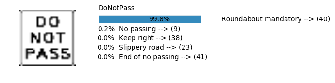
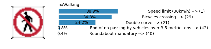
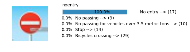

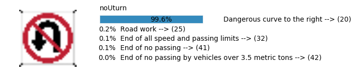
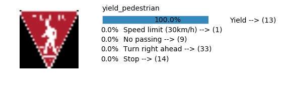
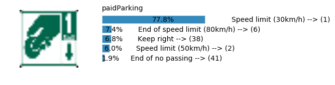
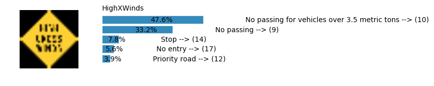
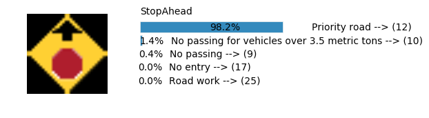

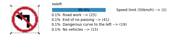
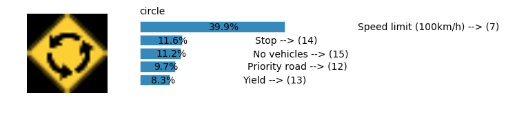
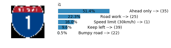

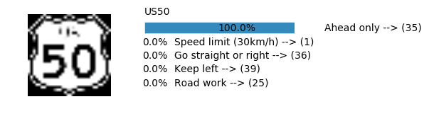

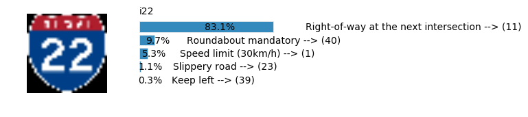
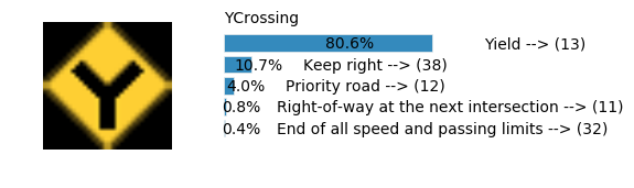
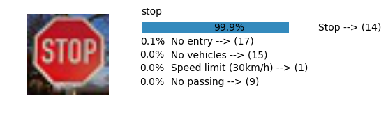
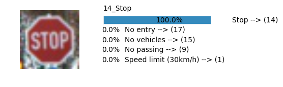
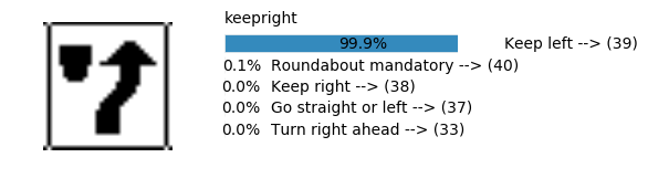
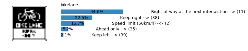
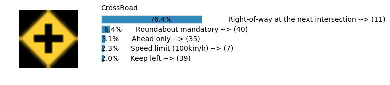
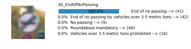
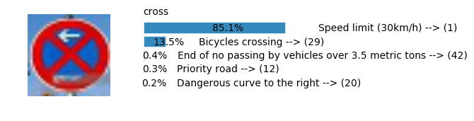
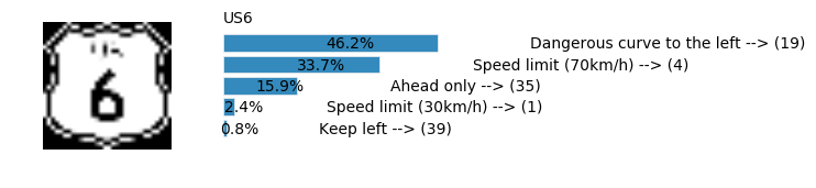
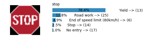
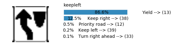
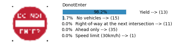
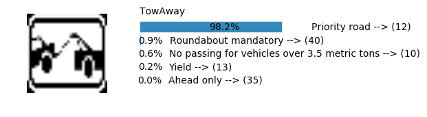
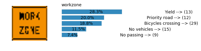
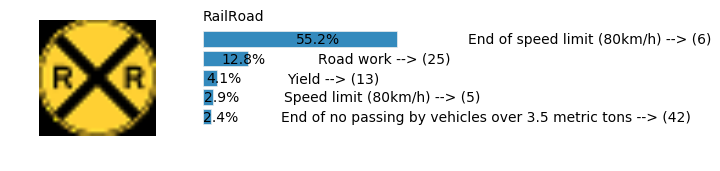
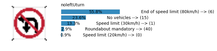

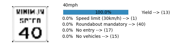
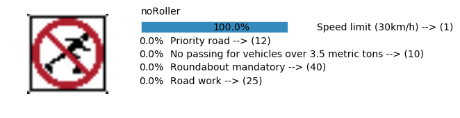
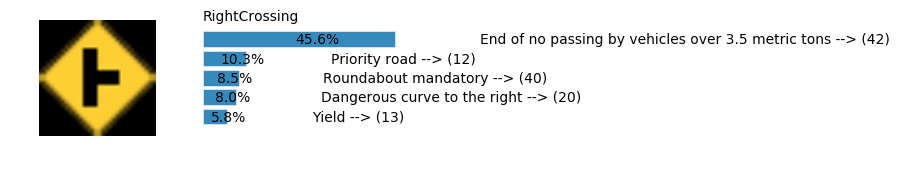
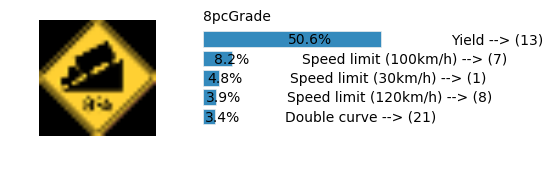
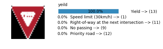
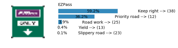
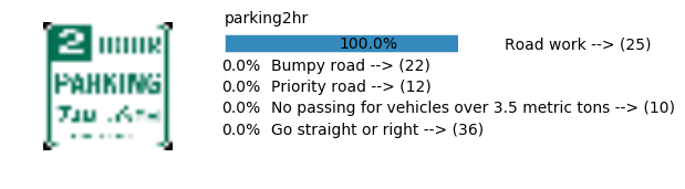

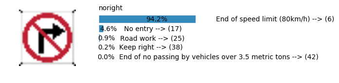
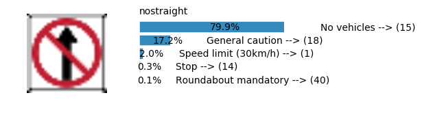
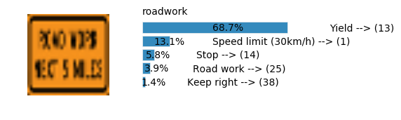
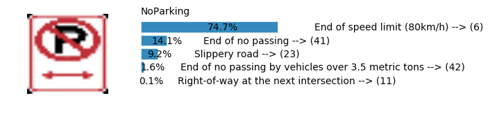
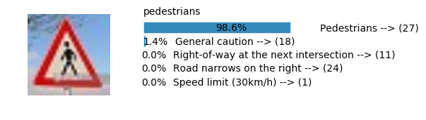
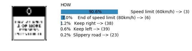
Accuracy
- Validation Accuracy: ~99%
- Testing Accuracy: 95.1%
- Real World Accuracy: 11 out of 48 images (~23%)
The reason the network didn’t perform well on these images is because signs of these categories were not included in the training set.
DeepNet No Merge Layers Prediction
sess, lenet_tensor_ops, data, cfg = train_and_test(preprocess=False, dropout_keep_prob = 0.75, epochs=50, network="deepnet", use_augmented_file=False)
predict(sess, lenet_tensor_ops, data.images_from_internet, data, cfg, top_k=5)
Predicting from Random Images: Number of Images: 48
(48, 32, 32, 3)
[[  4.96320635e-01   5.18143550e-02   4.18583900e-02   2.62362845e-02
    2.36967895e-02]
 [  7.58150160e-01   3.11358031e-02   2.40883417e-02   1.52391000e-02
    1.44358482e-02]
 [  1.00000000e+00   1.71898942e-15   3.28273740e-17   2.08940570e-18
    6.52752520e-19]
 [  6.50650203e-01   2.57410407e-01   4.97051254e-02   4.53829300e-03
    3.82647454e-03]
 [  1.74307853e-01   1.45416841e-01   7.15072528e-02   6.10274263e-02
    4.24179807e-02]
 [  2.53697395e-01   6.57131448e-02   4.93942462e-02   4.79025505e-02
    3.26466560e-02]
 [  9.98047948e-01   8.05428659e-04   5.80315245e-04   1.91798768e-04
    1.29238557e-04]
 [  1.80933833e-01   8.51858854e-02   6.94965050e-02   5.66996112e-02
    4.05882262e-02]
 [  9.31055546e-02   6.17452860e-02   5.75389527e-02   5.00681438e-02
    4.47426699e-02]
 [  1.00000000e+00   9.23194692e-18   2.27498657e-18   2.25448464e-19
    1.42598661e-19]
 [  3.49201798e-01   1.63566038e-01   5.28052896e-02   4.05855998e-02
    3.84167880e-02]
 [  9.40003544e-02   6.97816014e-02   5.43987155e-02   4.46421020e-02
    4.45429385e-02]
 [  1.00000000e+00   3.89672572e-10   2.95923980e-11   1.60349967e-12
    2.07540243e-13]
 [  8.38552952e-01   3.39123048e-02   2.16210373e-02   2.15000305e-02
    2.10180283e-02]
 [  5.07503510e-01   2.06898913e-01   3.61549854e-02   2.07158979e-02
    1.85478851e-02]
 [  6.41178191e-01   5.11642806e-02   4.15577143e-02   3.94946635e-02
    3.13082226e-02]
 [  5.43202795e-02   4.53511626e-02   4.45044897e-02   4.15787622e-02
    3.93682346e-02]
 [  7.85933256e-01   7.82854408e-02   2.59162951e-02   1.71977468e-02
    1.15314787e-02]
 [  9.89452124e-01   3.08159157e-03   2.07610079e-03   8.96831509e-04
    5.93360397e-04]
 [  9.99995232e-01   2.50080438e-06   1.17486320e-06   2.94505384e-07
    2.87629916e-07]
 [  9.99439061e-01   3.00879328e-04   5.84091722e-05   4.96795001e-05
    2.83852460e-05]
 [  1.31927878e-01   7.09761903e-02   7.07011670e-02   5.87634705e-02
    3.61877568e-02]
 [  2.93491602e-01   1.22236080e-01   3.98875512e-02   2.99449768e-02
    2.86520980e-02]
 [  1.00000000e+00   6.01612672e-14   1.01885273e-14   1.05613394e-15
    7.20465367e-16]
 [  1.25516951e-01   1.00832604e-01   7.61220306e-02   7.46601075e-02
    6.08591624e-02]
 [  5.31519473e-01   2.41912842e-01   4.99162190e-02   4.84670326e-02
    2.94072554e-02]
 [  9.61579621e-01   9.53180250e-03   5.91292745e-03   3.42027331e-03
    2.04818044e-03]
 [  1.91623643e-01   1.03008941e-01   7.83773959e-02   4.99154478e-02
    4.57430407e-02]
 [  9.99999404e-01   6.16566581e-07   1.83481230e-08   8.22325852e-09
    3.64568198e-09]
 [  6.59924388e-01   5.13115525e-02   3.44394334e-02   3.29011641e-02
    1.41200516e-02]
 [  1.65159732e-01   8.12835321e-02   4.97879684e-02   4.86464426e-02
    3.63697708e-02]
 [  7.04663619e-02   4.35333401e-02   4.35010903e-02   3.76710482e-02
    3.32230181e-02]
 [  1.75844282e-01   1.64255053e-01   4.99467514e-02   4.68471311e-02
    4.04395387e-02]
 [  1.00000000e+00   2.06628476e-18   2.19155546e-21   1.68265864e-21
    1.20272546e-21]
 [  9.44414854e-01   3.51007320e-02   4.77679307e-03   3.90309468e-03
    2.36888579e-03]
 [  3.53563011e-01   8.28672796e-02   5.17377034e-02   4.58230935e-02
    3.39295380e-02]
 [  9.47003245e-01   2.60775052e-02   1.47607662e-02   6.25074841e-03
    1.69483759e-03]
 [  2.15507433e-01   3.79748680e-02   3.66961658e-02   3.45788263e-02
    3.40154693e-02]
 [  9.84030962e-01   3.64439352e-03   2.61146622e-03   2.11428734e-03
    1.33312854e-03]
 [  2.33299598e-01   9.57155749e-02   4.79845218e-02   4.68197539e-02
    4.48211208e-02]
 [  1.38407663e-01   5.21076024e-02   5.08718528e-02   4.39307541e-02
    4.27807979e-02]
 [  9.96550798e-01   1.16964069e-03   6.67734887e-04   6.56474556e-04
    3.77771386e-04]
 [  5.53242624e-01   8.51595774e-02   3.52896042e-02   2.25436669e-02
    1.95045080e-02]
 [  9.96968329e-01   1.12940767e-03   4.29547654e-04   2.92290380e-04
    1.27864027e-04]
 [  7.45210722e-02   6.76817521e-02   5.19191921e-02   4.79956269e-02
    4.48146462e-02]
 [  1.00000000e+00   7.10589157e-11   2.82271411e-11   5.72655584e-13
    3.22633142e-13]
 [  9.99996543e-01   9.82874553e-07   9.04527440e-07   8.42212273e-07
    4.42830014e-07]
 [  9.93906081e-01   1.90753699e-03   7.34885398e-04   3.64089647e-04
    3.11268290e-04]] [[11 26 30 27 23]
 [27 20 11 24 26]
 [17 15  1  7  5]
 [28 23 29 10 17]
 [ 1  4 19  0 13]
 [ 3  2  5 13 38]
 [40 38 36 33 37]
 [ 2  5 37  1 18]
 [14 26 37 18 31]
 [13  1 19  0 24]
 [40  2 38 18 39]
 [26 37 25 14 18]
 [35 36 34 39 10]
 [ 5  1  7  2  3]
 [ 2  6  1 11 20]
 [34  9 33 35 28]
 [ 2 14 37 29 10]
 [ 7 40  8  5 38]
 [14 37 26 18 17]
 [14 37 26 17 18]
 [11 30 26 23 33]
 [40  2 36 37 38]
 [ 9  8 16 13 15]
 [41 32 16 22 33]
 [36 38 34 33 35]
 [ 4  7  1 15  8]
 [14 37 26 18 17]
 [29 13 28  2 17]
 [17 15  1 29  7]
 [13  2  1  3 10]
 [21 31 18 29 19]
 [ 1  2  5  4 15]
 [28  9  8 29  0]
 [ 2  1 40  6  3]
 [ 4  1  0 15  8]
 [21 31 33 29 10]
 [ 8  5  7  4 15]
 [ 9  8  2 16 15]
 [13 10 28  1 17]
 [17 29 21 15  2]
 [40  2 36 38 11]
 [35  8 33 34 36]
 [ 9  2  8  6 39]
 [11 30 26 27 23]
 [21 31 18 37  2]
 [ 9 16  8 13 41]
 [27 20 11 24 22]
 [11 30 26 27 33]]

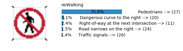
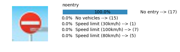
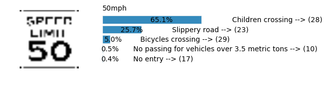
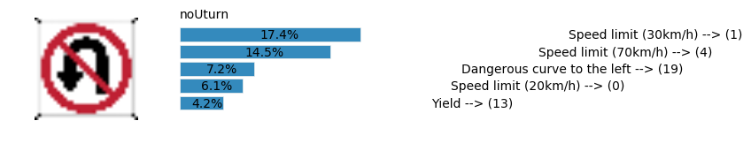
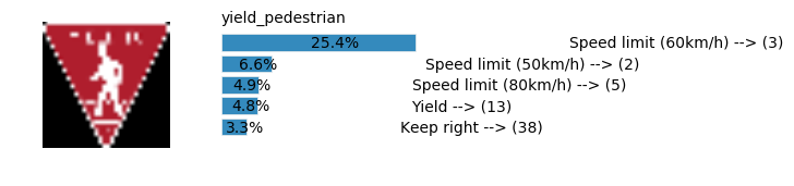

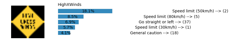
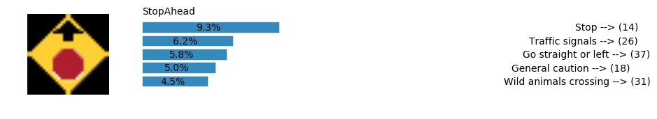
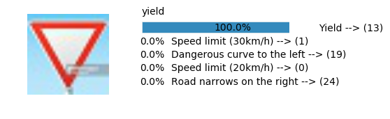
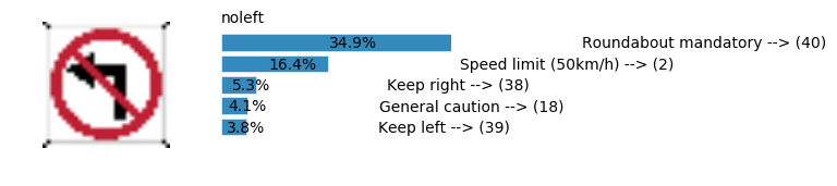
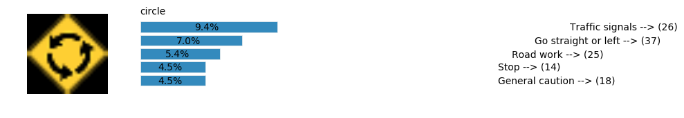
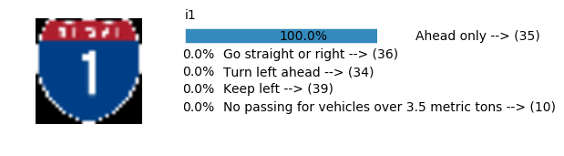
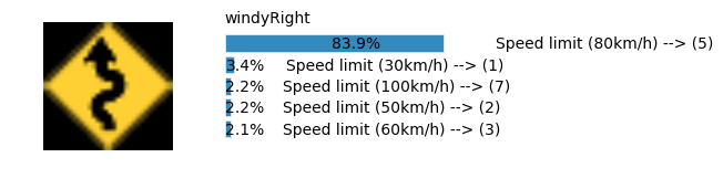
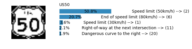

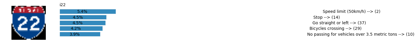
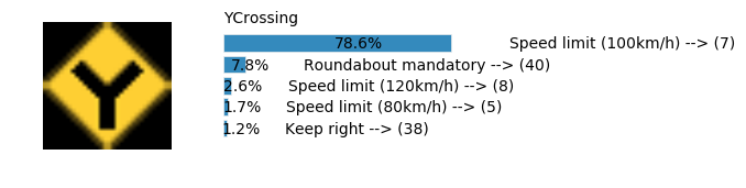
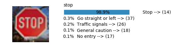
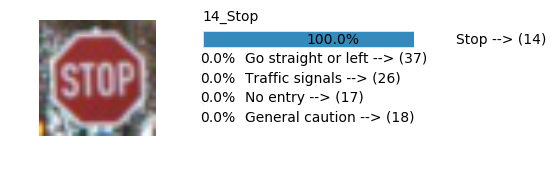
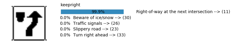
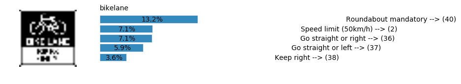
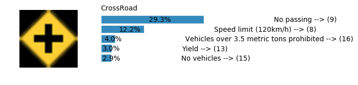
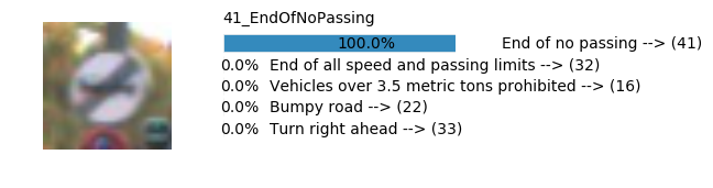
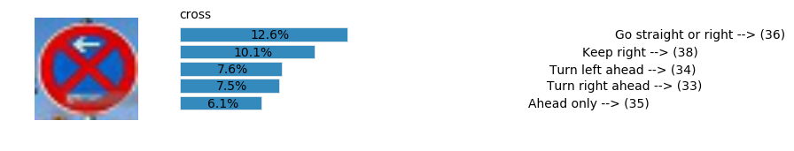
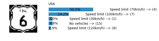
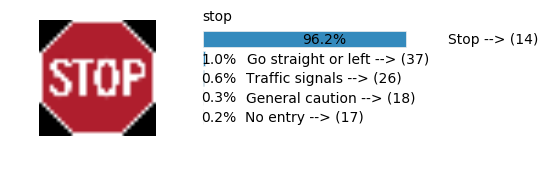

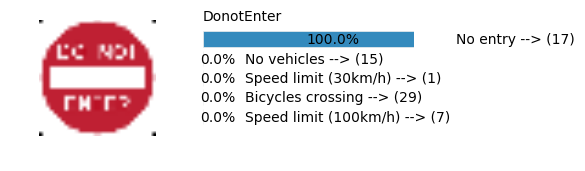
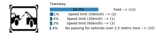
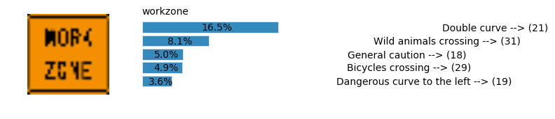
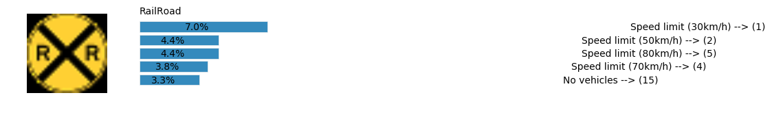
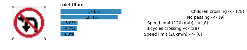
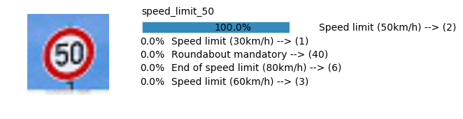
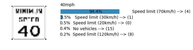
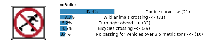
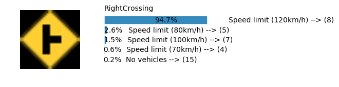
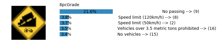
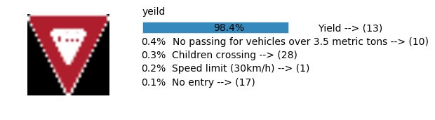
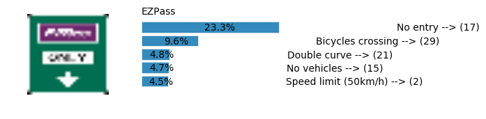
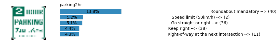
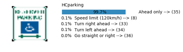
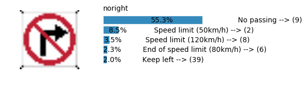
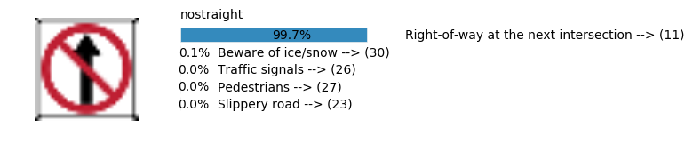
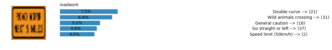
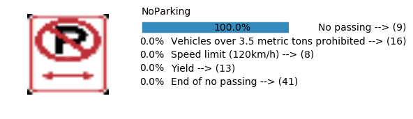
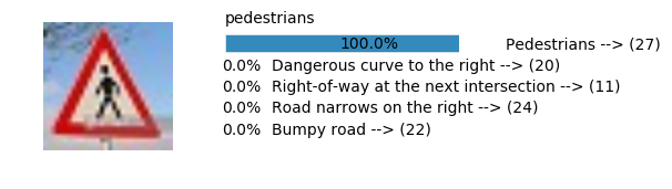
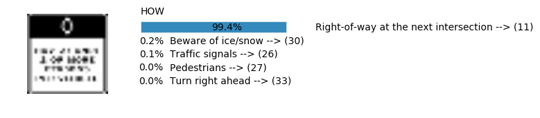
Accuracy
- The data for this model got erased accidently and I didn’t get a chance to rerun the model. However, I had the session still active to run the model.
- Real World Accuracy: 11 out of 48 images (~23%)
The reason the network didn’t perform well on these images is because signs of these categories were not included in the training set.
Overall Thoughts on Results
The low accuracy on real world dataset is not very disheartening in this case because of the fact that these are completely new labels which the network hasn’t been trained on before. However, it would be interesting to find more images which include background, different lighting conditions (eg. night, rain, snow etc). It would also be important to see how if more similar signs from other countries can be closely identified with one of the labels currently trained on. Another thing to note is that the images are not very high resolution which could become a problem. It would also increase training time.
Step 4: Visualize the Neural Network’s State with Test Images
This Section is not required to complete but acts as an additional excersise for understaning the output of a neural network’s weights. While neural networks can be a great learning device they are often referred to as a black box. We can understand what the weights of a neural network look like better by plotting their feature maps. After successfully training your neural network you can see what it’s feature maps look like by plotting the output of the network’s weight layers in response to a test stimuli image. From these plotted feature maps, it’s possible to see what characteristics of an image the network finds interesting. For a sign, maybe the inner network feature maps react with high activation to the sign’s boundary outline or to the contrast in the sign’s painted symbol.
Provided for you below is the function code that allows you to get the visualization output of any tensorflow weight layer you want. The inputs to the function should be a stimuli image, one used during training or a new one you provided, and then the tensorflow variable name that represents the layer’s state during the training process, for instance if you wanted to see what the LeNet lab’s feature maps looked like for it’s second convolutional layer you could enter conv2 as the tf_activation variable.
For an example of what feature map outputs look like, check out NVIDIA’s results in their paper End-to-End Deep Learning for Self-Driving Cars in the section Visualization of internal CNN State. NVIDIA was able to show that their network’s inner weights had high activations to road boundary lines by comparing feature maps from an image with a clear path to one without. Try experimenting with a similar test to show that your trained network’s weights are looking for interesting features, whether it’s looking at differences in feature maps from images with or without a sign, or even what feature maps look like in a trained network vs a completely untrained one on the same sign image.

Your output should look something like this (above)
### Visualize your network's feature maps here.
### Feel free to use as many code cells as needed.

# image_input: the test image being fed into the network to produce the feature maps
# tf_activation: should be a tf variable name used during your training procedure that represents the calculated state of a specific weight layer
# activation_min/max: can be used to view the activation contrast in more detail, by default matplot sets min and max to the actual min and max values of the output
# plt_num: used to plot out multiple different weight feature map sets on the same block, just extend the plt number for each new feature map entry

def outputFeatureMap(sess, tensor_ops, image_input, tf_activation, activation_min=-1, activation_max=-1 ,plt_num=1):
    # Here make sure to preprocess your image_input in a way your network expects
    # with size, normalization, ect if needed
    # image_input =
    # Note: x should be the same name as your network's tensorflow data placeholder variable
    # If you get an error tf_activation is not defined it maybe having trouble accessing the variable from inside a function
    print(tf_activation)
    activation = tf_activation.eval(session=sess,feed_dict={tensor_ops.x : image_input, tensor_ops.dropout_keep_prob: 1.0})
    featuremaps = activation.shape[3]
    plt.figure(plt_num, figsize=(15,15))
    for featuremap in range(featuremaps):
        plt.subplot(6,8, featuremap+1) # sets the number of feature maps to show on each row and column
        plt.title('FeatureMap ' + str(featuremap)) # displays the feature map number
        if activation_min != -1 & activation_max != -1:
            plt.imshow(activation[0,:,:, featuremap], interpolation="nearest", vmin =activation_min, vmax=activation_max, cmap="gray")
        elif activation_max != -1:
            plt.imshow(activation[0,:,:, featuremap], interpolation="nearest", vmax=activation_max, cmap="gray")
        elif activation_min !=-1:
            plt.imshow(activation[0,:,:, featuremap], interpolation="nearest", vmin=activation_min, cmap="gray")
        else:
            plt.imshow(activation[0,:,:, featuremap], interpolation="nearest", cmap="gray")
# sess, tensor_ops, data, cfg = train_and_test(preprocess=False, epochs=100, network="lenet_udacity", use_augmented_file=False)
# Picking the Stop sign from the training dataset
stop_indices = np.where(data.y_train == 14)[0]
img = data.X_train[np.random.choice(stop_indices)]
plt.imshow(img)
<matplotlib.image.AxesImage at 0x7fb97a9bdfd0>
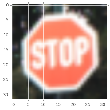
imgs = np.array([img])
outputFeatureMap(sess, tensor_ops, imgs, cfg.NETWORK_PARAMS["conv2"])
Tensor("add_45:0", shape=(?, 10, 10, 16), dtype=float32)
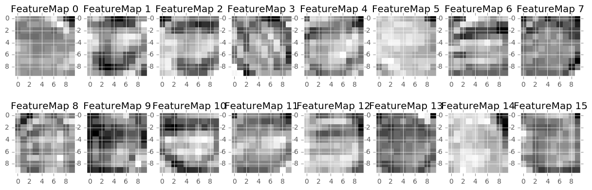
Question 9
Discuss how you used the visual output of your trained network’s feature maps to show that it had learned to look for interesting characteristics in traffic sign images
Answer: From the images above its really hard to tell what we are viewing so I couldn’t use anything from the feature maps.
Note: Once you have completed all of the code implementations and successfully answered each question above, you may finalize your work by exporting the iPython Notebook as an HTML document. You can do this by using the menu above and navigating to \n”, “File -> Download as -> HTML (.html). Include the finished document along with this notebook as your submission.
Project Writeup
Once you have completed the code implementation, document your results in a project writeup using this template as a guide. The writeup can be in a markdown or pdf file.
References
- Test Images source: Internet & https://github.com/vxy10/p2-TrafficSigns/tree/master/new_signs
- Code for the image preprocessing has been taken from internet.