Robust Lane Finding Algorithm

Introduction

Lane finding is an important algorithm for autonomous vehicles especially in high traffic areas where the margin of error is very low. Keeping true to the lane is important for the car and this problem has many implications. Udacity’s first project for lane finding from the Self Driving Car Nanodegree was an excellent introduction to this topic but it quickly made me realize how fragile the whole system was and how quickly the algorithm starts to fail. This was the 2nd project which explores the topic further by using some more advanced topics as compared to what was presented in the first project.

The project revolves around finding lanes by a camera which is mounted at the center of the car. The code is in lane_line_detection.py and the code can be run with the following command line.

python lane_line_detection.py --pipeline video --file project_video.mp4 --frames 3

The project also consists of other commands line options which can be used to control the behavior of the project.

Algorithm Overview

The algorithm starts with first performing offline steps i.e. performing Camera Calibration. Lens typically have distortions and it is necessary to perform distortion correction for the lens before the images from the camera can be further processed.

Offline Camera Calibration Steps:

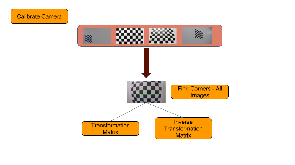
The diagram above shows a brief overview of how the camera calibration is performed. Multiple images of a known size chess board is first used. Objects points are passed in which get mapped to the images to eventually find the corner points on them. As these are found, a matrix is accumulated which essentially is the camera calibration matrix.

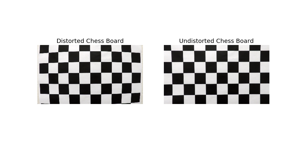
This matrix is multiplied to every incoming image to undistort it.

Real time Processing Steps:

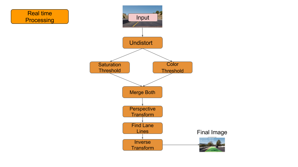
The steps shown here represent the overall algorithm which is used to find out the lane lines. These have to run in real time so it is very important to keep in mind the processing cost of any associated steps that are there and any step that could be parallelized.

1) Initial Input Image provided 2) Un-distort based on Camera Calibration 3) Perform Saturation Thresholding 4) Perform Color thresholding 5) Merge the 2 thresholded images to extract the white & yellow lane markings on the road 6) Define Region of Interest 7) Perform Perspective Transformation to convert to bird’s eye view. 8) Find areas of interest on the images by figuring out pixel intensities and fit a polynomial to it 9) Mark the region on birds-eye view and perform inverse transform to project on initial undistorted image

Undistortion

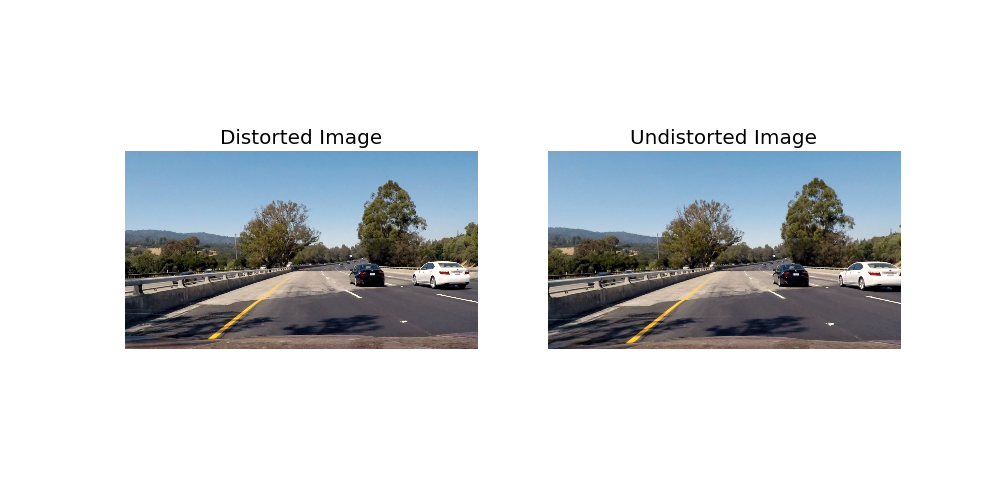
The undistortion is performed by multiplying the transformation matrix we obtained from the camera calibration. The image below shows the result from the un-distortion from the camera calibration matrix.

The class CameraCalibration has methods which store the calibration file once its calibrated and also has the methods to load and calibrate the camera.

Saturation Thresholding

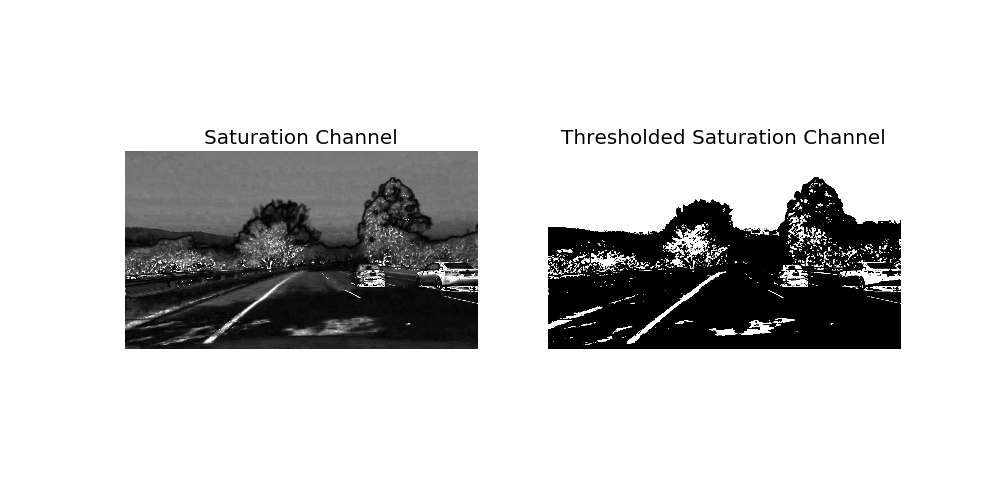
Yellow color lanes are best extracted by doing thresholding on the saturation images. So once we have the un-distorted images we convert it to HLS image. I use a thresholding values of (90, 255) to extract the yellow lines from the image. The image below shows both the saturation channel and the yellow line extracted.

The Thresholder class is responsible for having all the methods for thresholding. Thresholder::simple_threshold is used for doing threshold on the saturation channel.

Color Thresholding & Merging

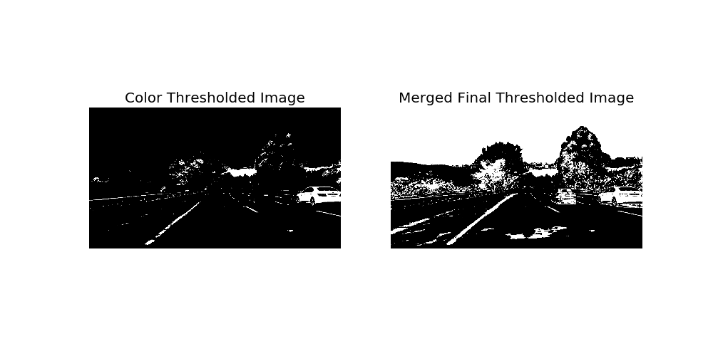
I tried doing a combined thresholding to extract the white lane lines but the results weren’t as well. So I do a Color thresholding by first converting the image to HSV. I use different ranges of whites to extract the lanes. The code below shows the thresholds used to compute the color thresholds.

sensitivity_1 = 68
white = cv2.inRange(hsv, (0, 0, 255 - sensitivity_1), (255, 20, 255))

sensitivity_2 = 60
hsl = cv2.cvtColor(img, cv2.COLOR_RGB2HLS)
white_2 = cv2.inRange(hsl, (0, 255 - sensitivity_2, 0), (255, 255, sensitivity_2))
white_3 = cv2.inRange(img, (200, 200, 200), (255, 255, 255))

The color threshold is then combined with the saturation thresholded image to generate a merged image which extracts the best of both worlds.

This code is present in the Thresholder::color_threshold method.

Region of Interest

During this step we define a region of interest. This is essentially the region which defines the perspective image of the road and the lanes. However we want a top view where the road looks like it is being seen from the top of the road. The image below shows the region of interest and what it is transformed to.

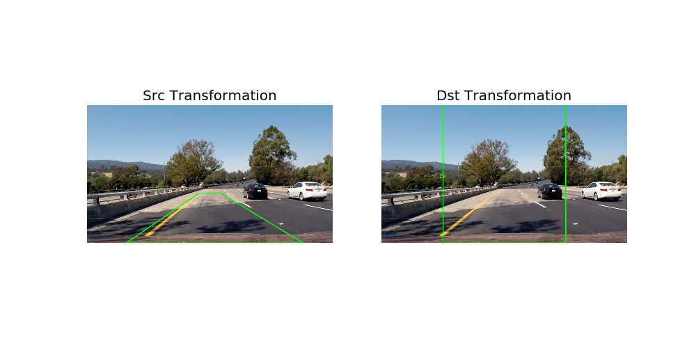
With these regions defined we create a perspective transform and we get a transformation matrix and an inverse transformation matrix. The inverse transformation matrix is used at the last step to transform the perspective image back to the original image.

The code for this part is present in RegionOfInterest::warp_perspective_to_top_down

Lane Finding Algorithm

The image below shows the perspective image. This image shows the bird’s eye view of the road.

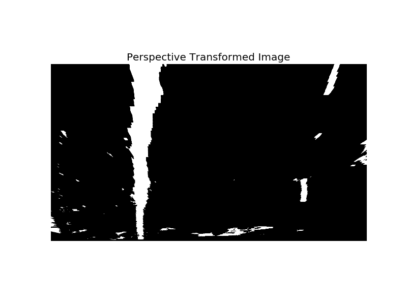
The basic idea of the algorithm is very similar to the first project of the Lane finding algorithm. In that project we used Hough transform to find out the lines from the binary images and then use a straight line fitting to generate the lane line. That algorithm didn’t perform very well with curved roads. This algorithm however takes a more intuitive approach to find lane lines.

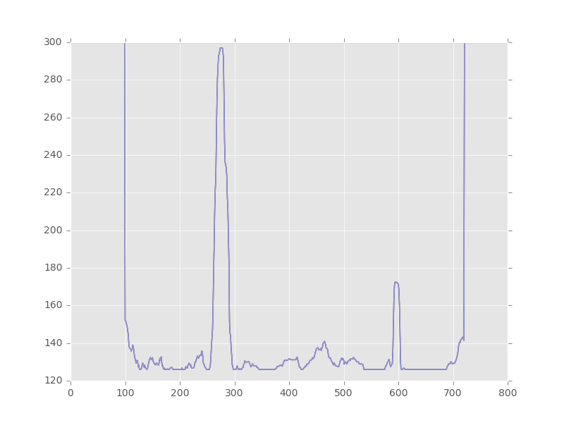
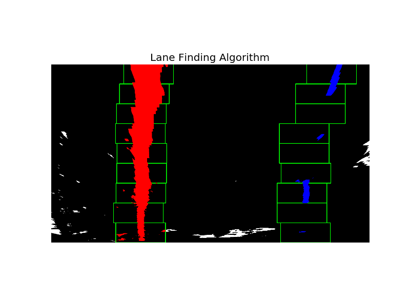
The first step is to do a histogram on the bottom half of the image to find the high intensities i.e. the white pixels on the image. Once we have the histogram, a window of 100 pixels x 100 pixels is used. The bottom image shows the algorithm as it proceeds. For every window the mean of the pixels is computed and then that is used to search the next window in the pixel image.

Once this entire process completes, the algorithm figures out the major chunk of pixels. Once we have the left lane pixels and the right lane pixels a polynomial fitting is performed.

After computing the lanes, we draw them back on the original undistorted image as follows.

Fine tuning:

• Tried constraining the polyline fit to the center of the box searches but that didn’t work out well.
• Frame averaging - Took about 10 previous frames data to average and get a smooth polyline. This seemed to work decently well for the challenge video.

This part of the algorithm is present in LaneFinder::full_lane_finding_step

Short circuiting the lane finding algorithm

Once a full lane finding step is performed for the next frames the search is started around the lanes identified from the previous frame. However, if at any point either the left lane or right lane are not found by this approach a full search is performed. The partial lane finding code is present in LaneFinder::partial_lane_finding_step

Inverse Transform & Final Result

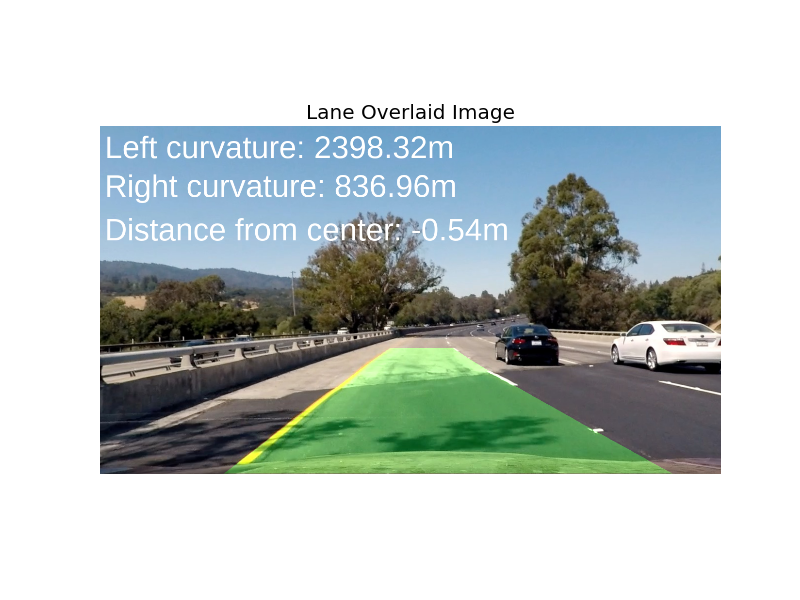Once the lanes line region is drawn on the perspective image, the inverse transformation matrix which was obtained when we went from the original image’s region of interest to the bird’s eye view. This gives the final lane finding image.

The final image overlay and visualization code is also contained in the LaneFinder class in the LaneFinder::overlay methods.

Computing the curvature

Computing the curvature involves computing the derivatives of the left lane and the right lane. Since we use a 2nd degree polynomial to fit the lines. The reason for using a 2nd degree polynomial was to fit the curves on the road. 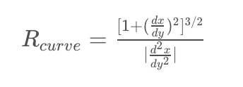The above equation is used to compute the curvature. 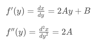The derivative values are the ones shown here and which is obtained from numpy. LaneFinder::compute_curvature

Distance from center

The equation for computing the distance from the center is as follows. ((B + C) / 2) - A where

• A - Dot product of the center point (height / 2, width) and TO_METER which is the transformation from pixel space to Meters.
• B - First order of derivative of left lane.
• C - First order of derivative of right lane. LaneFinder::distance_from_center

Problems with Algorithm

Simple Project Video:

The algorithm tried out in the above sections tend to work well with the project video and didn’t have any kind of project with the partial lane finding steps.

Challenge Video:

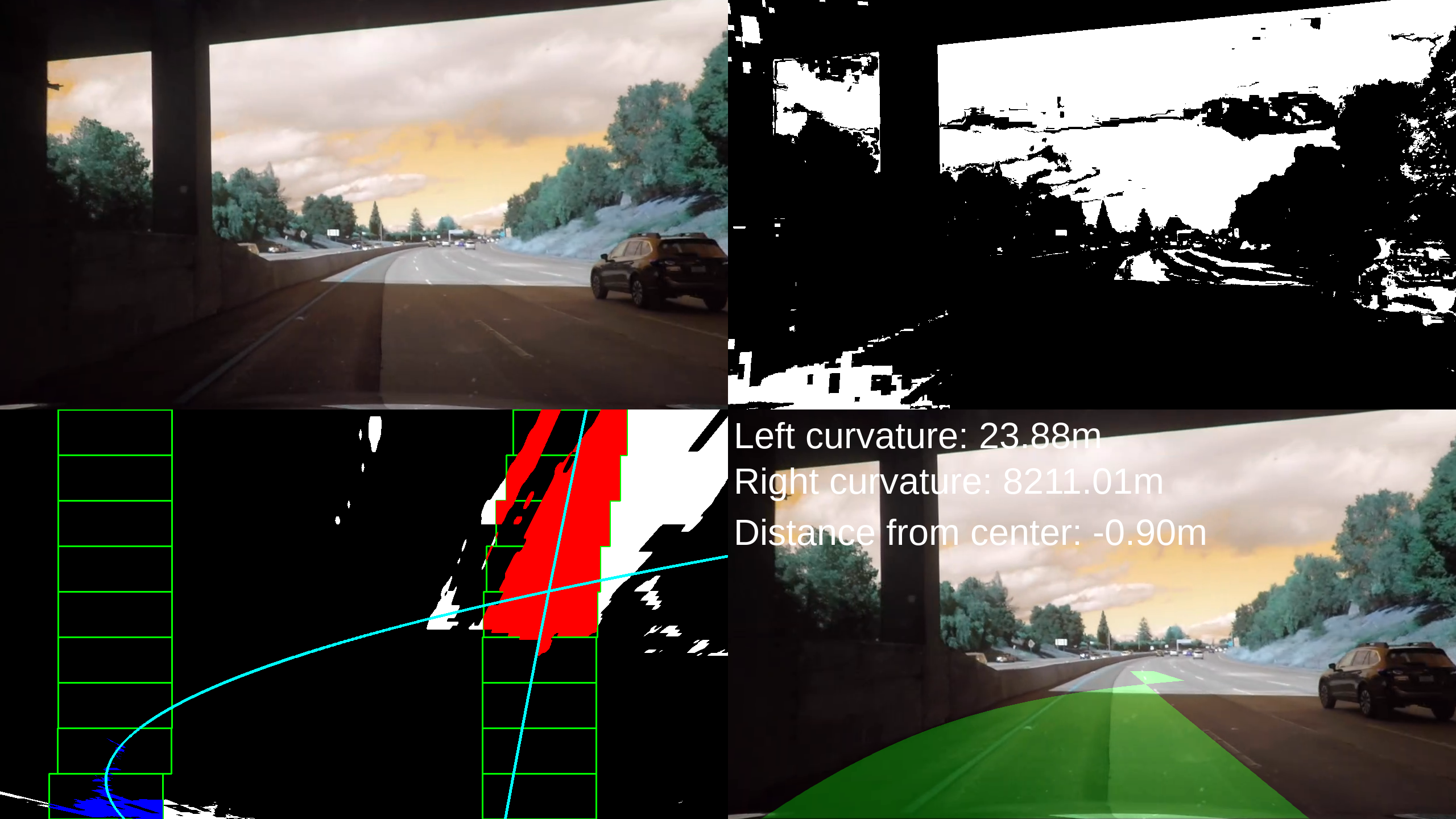
The biggest problem with the challenge video was the shadows under the bridge where the thresholding seems to detect either way too many regions or not detect the yellow lane lines properly.

Harder Challenge Video:

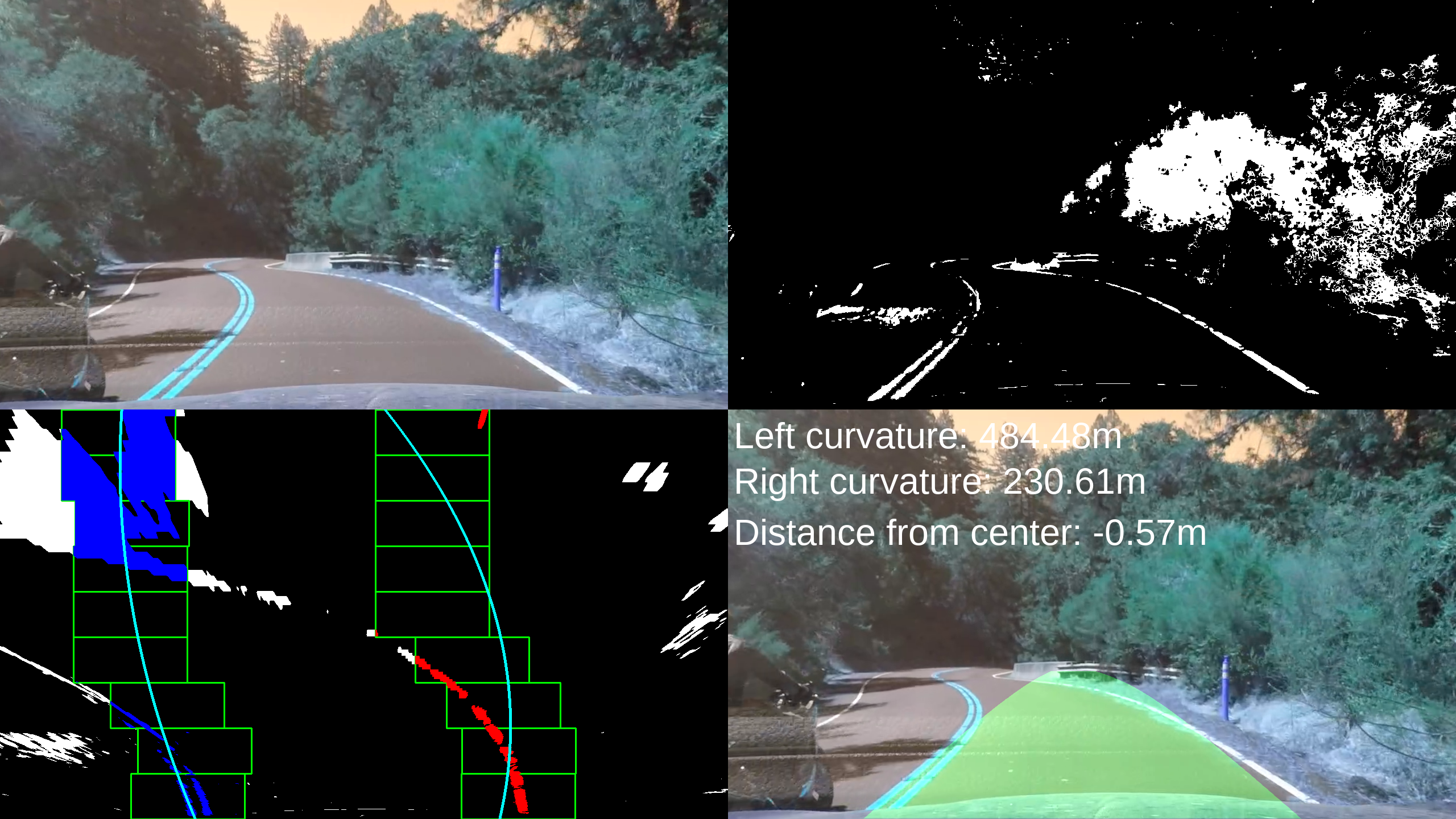
The harder challenge has a greater problem with the core algorithm itself. The problem is that the lane curves very highly. The problem why this becomes problematic is because the right lane curves into the region of the left lane and hence the right lane is mistakenly recognized as a part of the left lane.

Conclusion

Lane finding is definitely a hard problem which is pretty evident from just the input images provided so considering different lighting conditions and weather conditions as well as road conditions it could be extremely challenging to recognize lane lines accurately. I intend to return to the harder challenges and tweak the techniques to see if I can get a better solution by doing that.