PyVyM - A python based VM for 'Python'

Github Link

Finally after thinking and planning for a long time, I decided to start my blog and write about some of my tinkering. So here goes. :) This blog is about a simple process virtual machine written in python for python. There are some very good resources if you want to read up on python based vm’s. Here is a curated list to read about.

https://pythonguy.wordpress.com/2008/04/17/writing-a-virtual-machine-in-python/
http://rsms.me/2012/10/14/sol-a-sunny-little-virtual-machine.html
https://www.youtube.com/watch?v=HVUTjQzESeo

So what is a ‘Process’ Virtual Machine ?

Wikipedia defines a process virtual machine as follows: ‘process virtual machines are designed to execute a single computer program by providing an abstracted and platform-independent program execution environment.’ What does this mean ? It means that we emulate the behavior of the platform to run the program. Generally, VM’s target a specific language and emulate the bahavior of executing each instruction. So think of it as a glorified interpreter although there are some subtle differences. An interpreter is part of a virtual machine. For example, most of the java virtual machines come with interpreters and many with JIT compilers to accelerate frequently executed code. Java uses Java Virtual Machine (JVM) thus giving it the flexibility to run across platforms, since the difference in the platform is abstracted by the virtual machine. Similarly, C# uses Common Language Runtime (CLR) which is also a VM.

So what have I implemented ?

I enjoy writing python so I decided to write a virtual machine which could understand python code and execute it.

Introduction:

Overall Flow

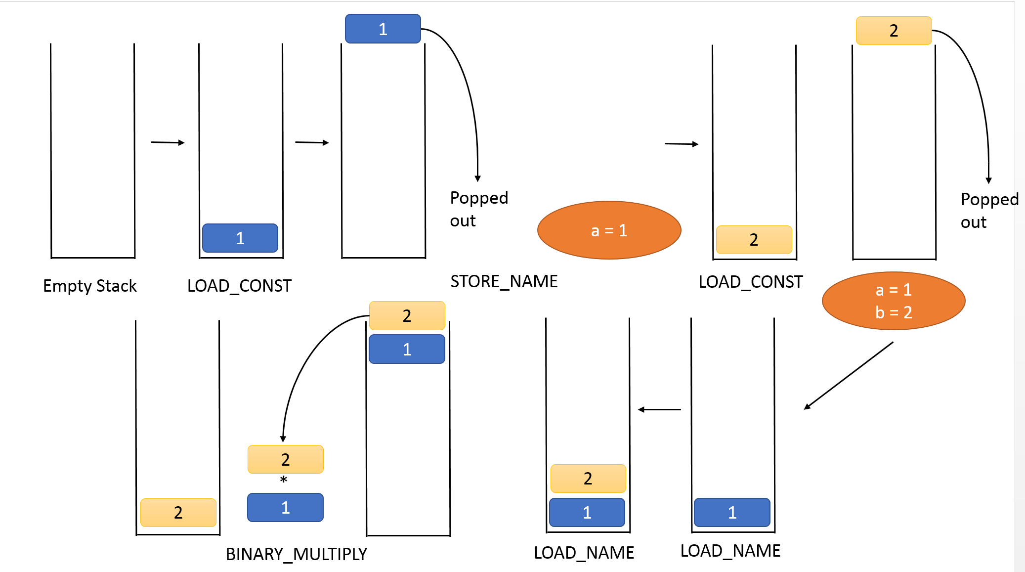
So the diagram above shows the overall flow of the VM. Python source is compiled by the python builtin compile method. Python generates what is called as bytecode. Essentially bytecode is a assembly version of code generated. It looks and feels like assembly. Python generated bytecode is a stack based machine which means that the operands of every operation are pushed onto a stack and then popped when the instruction is actually to be executed. A good instruction to stack based machines is presented in the Coursera Compilers course. Take a look if you are interested.

Python Bytecode structure

The youtube link at the top of the page gives an introduction to python bytecode and how they are used. I would rather start by giving examples to show what it means.

a = 1
b = 2
c = a * b

The code below shows the disassembly generated by python.

1           0 LOAD_CONST               0 (1)
            3 STORE_NAME               0 (a)

2           6 LOAD_CONST               1 (2)
            9 STORE_NAME               1 (b)

3          12 LOAD_NAME                0 (a)
           15 LOAD_NAME                1 (b)
           18 BINARY_MULTIPLY
           19 STORE_NAME               2 (c)
           22 LOAD_CONST               2 (None)
           25 RETURN_VALUE

So lets dissect this code. I have annotated the code below with what they mean. This can be easily achieved by storing this python code in a file and then read the file. The compile method returns a code object.

code object fields

co_argcount: number of arguments (not including * or ** args)
co_code: string of raw compiled bytecode
co_consts: tuple of constants used in the bytecode
co_filename: name of file in which this code object was created
co_firstlineno: number of first line in Python source code
co_flags: bitmap: 1=optimized 2=newlocals 4=*arg 8=**arg
co_lnotab: encoded mapping of line numbers to bytecode indices
co_name: name with which this code object was defined
co_names: tuple of names of local variables
co_nlocals: number of local variables
co_stacksize: virtual machine stack space required
co_varnames: tuple of names of arguments and local variables

I have annotated the bytecode below.

1 (LineNo corresponding to source)           0(ByteOffset) LOAD_CONST(Opcode)               0 (From Stack) (1) (Value annotated by dis)
            3 STORE_NAME               0 (a)

2           6 LOAD_CONST               1 (2)
            9 STORE_NAME               1 (b)

3          12 LOAD_NAME                0 (a)
           15 LOAD_NAME                1 (b)
           18 BINARY_MULTIPLY
           19 STORE_NAME               2 (c)
           22 LOAD_CONST               2 (None)
           25 RETURN_VALUE

Each instruction loads from a different field depending on the instruction. For example, STORE_NAME 1 means that it picks up the name from co_names[1].

The python dis module disassembly has a very good introduction on this topic. https://docs.python.org/2/library/dis.html

Trace the program

Execution Flow

1           0 LOAD_CONST               0 (1)

The line loads the value 1 onto the stack.

            3 STORE_NAME               0 (a)

Once the 1 is loaded onto the stack, the STORE_NAME first pops the value from the stack and then stores it into the variable ‘a’. Now ‘a’ is stored as a global in the module. Similarly, ‘b’ is also loaded.

3          12 LOAD_NAME                0 (a)
           15 LOAD_NAME                1 (b)
           18 BINARY_MULTIPLY

Now, ‘a’, ‘b’ are fetched from the global scope (the module) and then popped from the stack and used in the binary multiply operation. So in this case its ‘2’ * ‘1’ = ‘2’ so ‘2’ is stored back onto the stack.

           19 STORE_NAME               2 (c)

So ‘c’ is now stored in the global scope with the value 2.

22 LOAD_CONST               2 (None)
25 RETURN_VALUE

The last 3 lines indicate that the const ‘None’ is being loaded and that is the value the module is eventually returning.

This was a very simple example of how the execution flows. In the next blog we will look at the how the vm executes this same simple program.

Satyajit Sarangi